
Read · 1 min
By Alex Federspiel

+3 contributors
Contributors

Operations with Vectors
Addition
Given and let .
Then,
Subtraction
Given and let .
Then,
Scalar Multiplication
Given and scalar .
Then,
Magnitude
Given .
Then the magnitude of , or , is .
Read · 1 min
Given and let .
Then,
Given and let .
Then,
Given and scalar .
Then,
Given .
Then the magnitude of , or , is .
Many contest problems feel more like puzzles than homework. They are a good way to find out how much fun math can be. These are real problems from the AMC 12 and AIME, the national math competitions for middle and high school students, each with a worked solution on LIVE by Po-Shen Loh.
Video · + 1 min read
by Math and Stats Help

This video by Math and Stats Help reviews the basic operations that we can do with vectors.
Given and , find:
A)
B)
C)
Be mindful of the signs for the vector quantities.
We're going to look at A first. This is called scalar multiplication because we're looking at a scaled factor of . So, we're taking the vector, and multiplying it by .
We'll sort of use the distributive property to distribute the scaled factor of .
Now, let's look at B. Here, we will be adding, in addition to the scalar multiplication we saw earlier.
To add the two vectors together, you need to add corresponding elements.
Lastly, we will look at C. Here we see vector subtraction and scalar multiplication.
We still want to be aware of PEMDAS, so we're going to do the scalar multiplication first.
These are our resultant vectors:
A)
B)
C)
Illustrated · 1 min
There are four main operations that we can do with vectors.
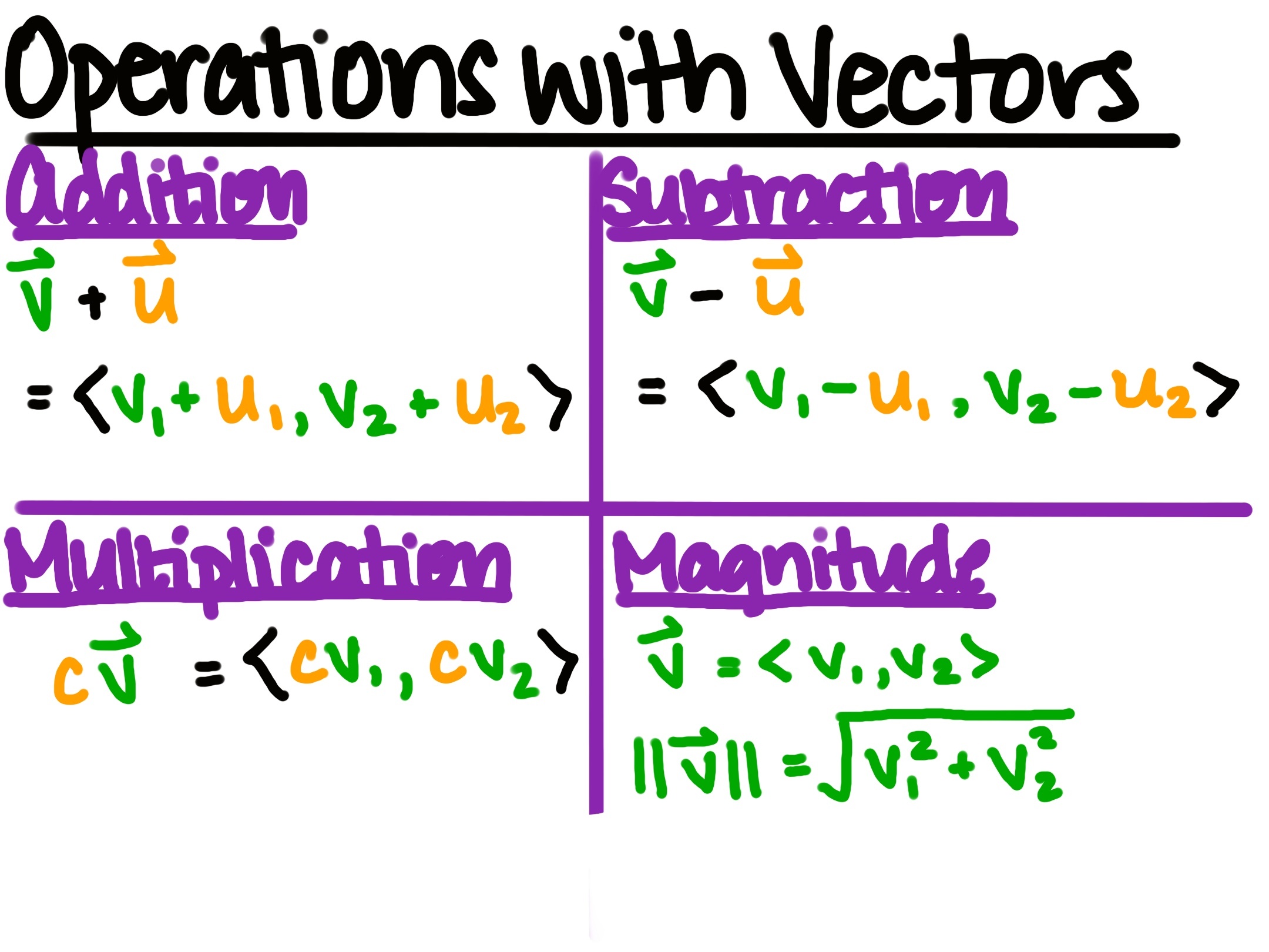
Image source: by Anusha Rahman
Vector-valued functions provide another way of parametrizing a curve by expressing position as a vector that changes with a parameter, often time. Instead of tracking each coordinate separately, the vector form captures both components together and makes operations like addition and scalar multiplication more intuitive. This perspective connects vector operations directly to motion and geometry, setting the stage for deeper work with parametric curves and vector functions.
Get ready to be a master of vectors! You can learn about the dot products, magnitude, the cross product, and vector projections.