তড়িৎ প্রবাহের সংজ্ঞা ও একক

Definition and Units of Current

Definition of Current(electric):

An electric current is a flow of electric charge.

Units of Current(electric):

The SI unit for measuring an electric current is the ampere, which is the flow of electric charge across a surface at the rate of one coulomb per second.

Introduction

Q: What is the first thing that happens when you power on your computer (or other electrical device)?

A: One simple answer is that energy is transferred from the energy source (e.g. battery or electrical mains supply) to the device. This energy transfer is usually mediated by an electric current.

Concept of Current

In plain mathematical terms, current is the rate of flow. This is quite a versatile concept, not restricted to electricity.

For a river, the flow rate (water current) can be defined as the volume of water passing through a certain point. On a smaller scale, we can think about a tap -- put a cup underneath and turn it on -- the flow rate might be something like one cup every ten seconds.

Current Equation

A simple equation to express this concept of "current as flow rate" is $$R=\frac{dQ}{dt}.$$ Here the symbol $Q$ represents the quantity of interest (e.g. volume of water, number of marbles, and so on) and $t$ represents time. This is an expression for the **instantaneous **flow rate $R$.

If we are just interested in the **average **flow rate, we can just calculate the total change in $Q$ divided by the total time interval, i.e. $$R=\frac{\Delta Q}{\Delta t}.$$

More Examples of Currents

Other than currents that stream quite continuously, like water and wind, we can also try to describe more granular (discrete) flows, like children going down a playground slide or marbles rolling on a ramp. In this section, let us look at some examples related to cars.

In a race like this Formula One race shown above, the "current" of cars is very irregular, depending on where and *when *you look to measure it. The concept of average current is more meaningful, and you can take this average by choosing a cross-section of the track (e.g. the finish line) and counting the number of cars that go by during a relatively long time interval.

As the density of cars increases, it becomes more meaningful to consider the current at different points of the road, and even over short intervals of time. It starts to make sense to try to describe the instantaneous current.

Basically, when it gets really crowded we will worry less about the granularity (discreteness) of the particles -- the situation becomes similar to how we imagine water to flow (thinking in terms of mass and volume rather than the actual molecules).

Electric Current

Let us now focus on electric currents in electrical circuits, which is the main topic of interest. The usual notation we use for current in this context is $I$, and the "quantity" symbol $Q$ represents electric charge. We write the current equation as $$I = \frac{dQ}{dt}.$$

Note that the SI unit for (electric) charge is the coulomb (C), and the SI unit for (electric) current is the ampere (A), both named after famous French scientists -- Charles Augustin de Coulomb (1736 – 1806) and André-Marie Ampère (1775 – 1836). The SI unit for time is the second (s).

Note further that we typically have quite a dense flow of charge so the idea of instantaneous electric current is usually not a problem (i.e. we can think of it as more similar to water flow than having a few cars racing along an extended circuit).

Charge Carriers

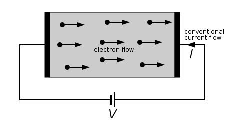
In metallic conductors, electric current is due to the flow of electrons, shown schematically in the Figure below. You may wish to note that in general, electric current is not always due to the flow of electrons (it could be due to the flow of ions in solution, for instance).

Current flow in a metallic conductor

You should be familiar with the basic idea from studying electrostatics that electric charges experience a force when placed in an electric field. When a battery drives current around a closed circuit, a simple picture of what happens physically is that the battery sets up an electric field throughout the circuit, which causes charges to experience forces and accelerate.

But just think about it for a moment and you might realise that what happens at the microscopic level is not going to be quite so simple. Nonetheless, we will stick to a classical (rather than a quantum) model. In this model, we imagine the metallic ions (e.g. copper ions for a copper wire) forming a solid lattice, with the conduction electrons forming a swirling sea around them. The conduction electrons experience electrostatic forces due to the rapidly varying and complicated field set up by the microscopic charge distribution within the metal.

Let us first consider the case of a piece of metal just sitting there without an external electric field being applied, before we move on to consider what happens when an electric field is applied (e.g. by connecting a battery in a closed circuit).

Without applied electric field

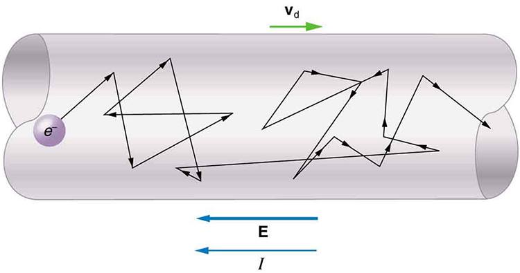
The beauty of all this complication is the essential randomness. If there is no reason for the conduction electrons to prefer one direction over another within the wire, then there is no net motion on average. This statement is fundamentally statistical in nature -- of course any particular conduction electron is going in some particular direction at some particular moment in time, but after averaging over its own historical trajectory and then averaging over many other conduction electrons, what we expect is that the entire sea of conduction electrons has moved without moving, as it were!

It is not completely wrong to think of the electrons in this situation without an applied electric field as an "ideal gas" of electrons, with the surface of the metal acting as the "walls" of the "container". Additionally, for metals, the typical velocity of conduction electrons is rather high, on the order of $10^6 \textrm{ m s}^{-1}$ (Neil W. Ashcroft and N. David Mermin, Solid state physics, Saunders College, 1976).

With electric field applied

The applied electric field now causes a systematic effect, in addition to the inherent randomness. When we apply an electric field across a metallic conductor (e.g. by connecting a battery in a closed circuit), there is an additional electrostatic force exerted on all the electric charges in the metal. The positive metal ions get pulled one way, and the conduction electrons experience a push in the other direction. The effect is microscopically minuscule but macroscopically significant, since there is an additional collective net motion experienced by all the charges! We describe the *average *net motion of the conduction electrons relative to the metallic ions as the drift velocity $v_d$.

Why a drift velocity and not acceleration?

If you're thinking about Newton's laws of motion, you might be wondering why the electric force does not cause the conduction electrons to keep accelerating and moving faster and faster. The short answer is that there are dissipative forces present -- energy is transferred to the metal, typically causing it to heat up. A steady supply of electrical power results in a steady current instead of a growing current!

The drift velocity is analogous to the terminal velocity experienced by a falling parachutist, though you might get quite confused trying to imagine the actual complicated motion of an electron!

Modelling drift velocity

To recap, our metal picture of current flow in a metallic conductor is a superposition of a net drift velocity for the conduction electrons and the "noise" of complicated and essentially random motion that occurs even without an applied electric field. And because that latter motion averages to zero, only the effect of collective drift is linked to current flow.

Thus, it makes sense to conceptually "ignore" the random motion and think only about the drift velocity, in order to visualise more intuitively what happens when a current flows. To build an intuition for electric currents, we now think about people walking (in a single direction only!) along a street.

Factors affecting electrical drift velocity

With this intuition from thinking about people walking, it is straightforward to see how electric currents can be similarly understood.

<>

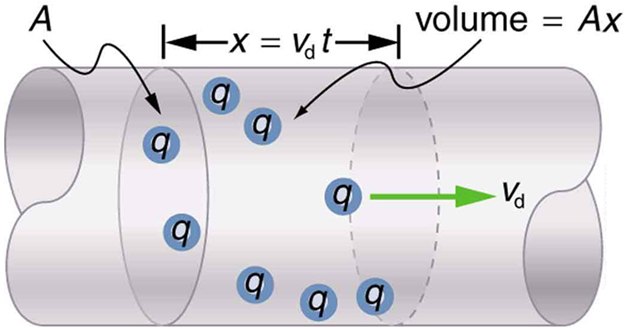
We can derive an expression for the drift velocity $v_d$ of the charge carriers within an electric circuit, based on this simple model. We start with the expression for the average current, $$I = \frac{\Delta Q}{\Delta t}$$ and think about how much charge $\Delta Q$ passes through a cross-section $A$ of the material (e.g. a wire) in the (short) time interval $\Delta t$.

At a particular point of the wire, all the charges in some volume $V = Ax$ will pass through after a time $\Delta t$, as shown in the Figure below.

To figure out the amount of charge that is contained in this volume $V$, we just have to count the number of charged carriers $N$ and multiply each according to the charge that it carries. We have $$\Delta Q = Nq,$$ where $q$ is the individual charge of each of these mobile carriers (assuming they are all the same, but this can be easily generalised if there are different types of charge carriers).

The number $N$ can also be related to the number density $n$ via $$n = \frac{N}{V}.$$ In other words, we multiply number density by the volume to get the total number, just like how we multiply mass density by the volume to get total mass. This number density of the charge carriers is usually quite uniform within a material, hence the utility of writing $N$ in terms of $n$.

We have $$\Delta Q = nqV,$$ so putting it all together, we have the expression for current as $$I = \frac{\Delta Q}{\Delta t} = nqA \frac{x}{\Delta t} = nqA v_d,$$ where $v_d = x / \Delta t$ is what we call the drift velocity. Notice that the drift velocity is higher when the wire is narrower -- otherwise there would be a "traffic jam" of electric charges that is unstable.

So in other places where the cross-section $A$ is higher, the length $x$ is shorter (so that the volume is the same). You would be intuitively familiar with this if you have ever used a finger to adjust the nozzle area of a water hose, or changed the setting on a shower head.

Notice that the drift velocity calculated is on the order of 0.1 millimetres per second! Nonetheless, electrical current flows very quickly, even through circuits spanning hundreds of kilometres, because of the collective motion of the conduction electrons as soon as the electric field is established in the circuit.

Current flow through semiconductors

Semiconductors played an integral part in the development of the transistor and the explosion of computer technology we have seen since then. While some ideas of quantum physics are crucial to appreciate what semiconductors are, in the context of drift velocity, the following "cartoon" model provides an impression.

<>

Semiconductors do not conduct electricity as well as metals, as they lack a "sea" of conduction electrons, but they still conduct electricity better than insulators. Generally, at higher temperatures, a semiconductor will have more mobile charge carriers that are able to contribute to the drift velocity. Interestingly, in some semiconductors, these charge carriers can behave like a (dilute) "gas" of electrons, while in others, these charge carriers are called "holes" as they behave effectively like a (dilute) gas of positively charged particles.

The number density $n$ of the mobile charge carriers can be changed by adding impurities -- the ability to do this is a key reason why semiconductors are so useful in technological applications. As this number density for semiconductors is several orders of magnitude smaller than for typical metals, the drift velocity in semiconductors is usually much higher.

Mechanical Model for Electric Current

There is a free journal article in Physics Education that introduces a mechanical model for electric current. The idea is that small marbles rolling down a ramp that is punctuated with heavy masses reproduces several of the features of electrical current in a metallic conductor.

Concluding remarks

We have considered the concept of current in the context of electricity, as well as more generally. We have also seen several formulations of the mathematical equation for current flow, such as the expression for instantaneous electric current $$I=\frac{dQ}{dt}$$ and a simpler one involving the average value of the current over a time interval, $Q=It$. We have also discussed the idea of drift velocity of mobile charge carriers, and gave a simple motivation for the equation $$I=n A v_d q.$$ Though we have not mentioned the concept of resistance explicitly, we saw briefly how energy is typically transferred to the conductor (e.g. causing heating effects) and thus a steady application of an electric field leads to a steady current.

Further exploration

As part of further exploration, you may also wish to consider a hands-on activity involving electrical conduction by coloured ions. Check out Episode 104-1 as part of the Teaching Advanced Physics website of the Institute of Physics.

A related YouTube video for this activity is found below. You may wish to make an estimate of the physical quantities involved!