রৈখিক ফাংশনের লেখের স্থানাঙ্কের তালিকা হতে লেখ অঙ্কন

Before this, knowঢাল-ইন্টারসেপ্ট আকার ($y = mx + b$)Function Notation - Definition & Examples

Illustrated · 1 min

Linear Functions

The name "linear functions" has the word "line" in it, which would suggest that, graphically, linear functions would look like lines.

And indeed they do. Here is a graph of: f(x)=−2x+3f(x)=-2x+3
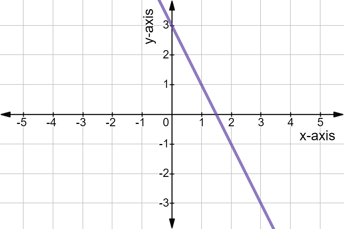
Graph of f(x) = -2x + 3.

Made using Desmos

Linear functions are straight lines because the function increases or decreases the same amount for every unit of change.

You'll see this a lot in science experiments, where there's a constant relationship between an independent variable and dependent variable.

Graphing Linear Functions

To graph linear functions, we need to plot at least 22 points and connect them. We can choose any two points on the line so the goal is to pick easy to find ones.

Let's see how with an example. Suppose we want to graph: f(x)=3x−5f(x)=3x-5 One of the easiest points to find is when x=0x=0; we can simply throw out the xx term. f(x)=3x−5f(0)=3(0)−5f(0)=−5\begin{align} f(x)&=3x-5\\ f({\color{#8925ae}{0}})&=3({\color{#8925ae}{0}})-5\\ f(0)&=-5 \end{align} We now have the point (0,−5)(0,-5).

The point (0,-5).

Made using Desmos

Choosing x=1x=1 for the second point is another easy calculation. f(x)=3x−5f(1)=3(1)−5f(1)=3−5f(1)=−2\begin{align} f(x)&=3x-5\\ f({\color{#8925ae}{1}})&=3({\color{#8925ae}{1}})-5\\ f(1)&=3-5\\ f(1)&=-2 \end{align} This gives us our second point of (1,−2)(1,-2).

The points (0,-5) and (1,-2).

Made using Desmos

This is all we need to graph the function. Just draw the line that passes through these two points.
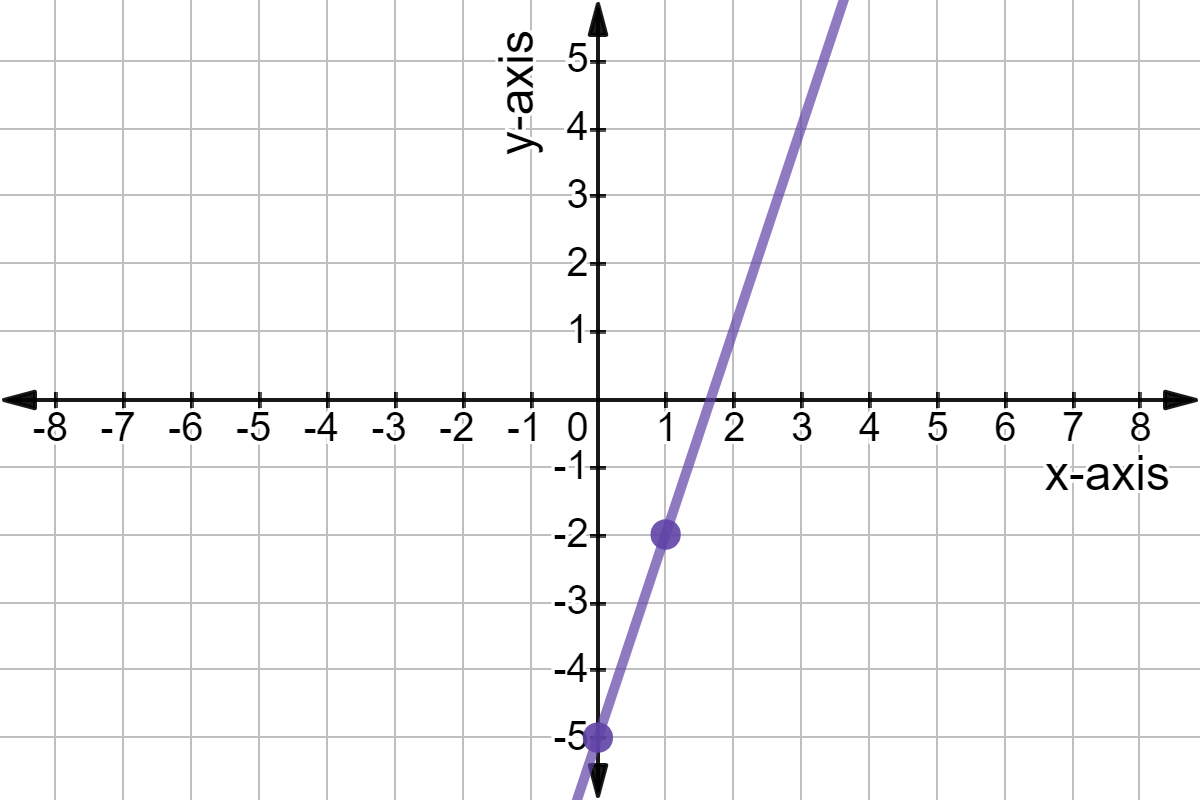
Graph of y = 3x - 5 with points (0,-5) and (1,-2).

Made using Desmos

Video · + 3 min read

(Video) Basic Linear Functions

by Math Antics

Here's a great video by Math Antics that teaches you about the graphs of linear functions. He explains how both the slope and yy-intercept affect how a graph looks.

Summary\large{\text{Summary}}

How to Graph a Linear Equation

Linear equations are very easy to graph. All you need is 22 points. The linear equation will always be the line that you make by connecting the points.

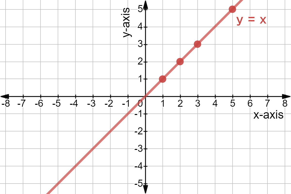
To find the points, we can use a table. Let's look at an example using the most basic linear equation: y=xy=x. This equation says that whatever our input xx is, our output yy will be the same thing. We set up our input-output table like so: xy\begin{array}{c|c} x&y\\ \hline \\ \\ \\ \end{array} Next, we write down some common input, xx, values to plug in. You only need two to construct the line, but for now we'll use more. xy1235\begin{array}{c|c} x&y\\ \hline 1&\\ 2&\\ 3&\\ 5& \end{array} Plug these xx values into our equation and solve to get their outputs or yy values. y=xy=1y=2y=3y=5\begin{align} y&=x\\ \hline y&=1\\ y&=2\\ y&=3\\ y&=5 \end{align} Because the input is equal to the output, we get the same numbers back out. Therefore, our table becomes: xy11223355\begin{array}{c|c} x&y\\ \hline 1&1\\ 2&2\\ 3&3\\ 5&5 \end{array} Let's plot these coordinates on a graph.

The points (1,1), (2,2), (3,3), and (5,5).

Made using Desmos

Finally, once you have your points, just draw a line through them to get the graph of the equation.

Graph of y = x.

Made using Desmos

y=mxy=mx

Here, we have a similar equation to before, but now there an extra variable, mm. For graphs, mm refers to the slope, or steepness. You'll learn how to calculate slope later, but for now let's see how it affects our graph.

When m=1m=1, our equation becomes: y=1xy=1x This is same as y=xy=x which is what we graphed before.

m>1m>1

When m=2m=2, our equation becomes: y=2xy=2x If we fill out an input table, we get: xy12243648\begin{array}{c|c} x&y\\ \hline 1&2\\ 2&4\\ 3&6\\ 4&8 \end{array} For every xx value, the yy value gets doubled. Plotting this, we get:

Graph of y = 2x with a reference of y = x.

Made using Desmos

This graph, is steeper than our previous one, which is in the background for reference.

As we pick larger and larger mm values, our graph gets steeper and steeper.

The lines y = x, y = 2x, y = 3x, and y = 10x.

Made using Desmos

As mm gets larger and larger, the line becomes more and more vertical. But, we can never reach perfectly vertical.

0<m<10<m<1

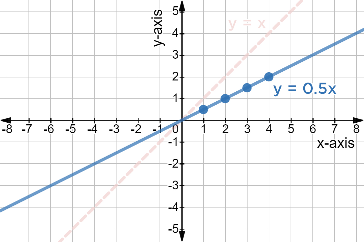
To get less steep graphs, we pick an mm that's between 00 and 11. Let's let m=12=0.5m=\frac12=0.5. Our input table gives us: xy10.52131.542\begin{array}{c|c} x&y\\ \hline 1&0.5\\ 2&1\\ 3&1.5\\ 4&2 \end{array} And our graph gives:

Graph of y = 1/2x with y = x as a reference.

Made using Desmos

As we choose mm's closer and closer to 00, our slope get's less and less steep.

Graphs of y = x, y = 1/2x, y = 1/4x, and y = 1/50x.

Made using Desmos

As mm gets closer to 00 the line becomes more and more horizontal. When m=0m=0, we do get a horizontal line.

m<0m<0

We can have negative slopes as well! These will appear as mirror images of their positive counterparts.

Let's look at m=−1m=-1. This gives us the equation: y=−1xy=-1x Our input table is: xy1−12−23−34−4\begin{array}{c|c} x&y\\ \hline 1&-1\\ 2&-2\\ 3&-3\\ 4&-4 \end{array} And our graph is:

Graph of y = -x with a reference of y = x.

Made using Desmos

Similarly, a more negative slope makes a more steeper line, and a negative slope closer to 00, makes a less steep line.

Graphs of y = -x, y = -2x, and y = -0.25x with references y = x, y = 2x, and y = 0.25x.

Made using Desmos

The Origin

No matter what we set mm to, our graphs will always have one point in common: the origin (0,0)(0,0).

A bunch of equations of the form y = mx. They all share the same point, the origin.

Made using Desmos

y=mx+by=mx+b

So what if we want a line that doesn't go through the origin? Well, we need to add a new variable, bb. y=mx+by=mx+b

To see what it does, let's start my letting m=1m=1. Our equation will then be y=x+by=x+b.

If we let b=1b=1, we have: y=x+1y=x+1 Our input table is: xy12233445\begin{array}{c|c} x&y\\ \hline 1&2\\ 2&3\\ 3&4\\ 4&5 \end{array} The graph looks like:

Graph of y = x + 1 with reference of y = x.

Made using Desmos

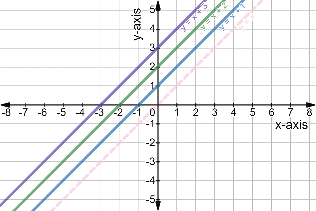
As you can see, this line is parallel to y=xy=x. If you look at where the point would cross the origin, (0,0)(0,0), it now crosses the point (0,1)(0,1). This 11 is what we set bb equal to.

Plugging in other values for bb, we get:

Graphs of y = x + 3, y = x + 2, and y = x + 1 with a reference of y = x.

Made using Desmos

Practice 1

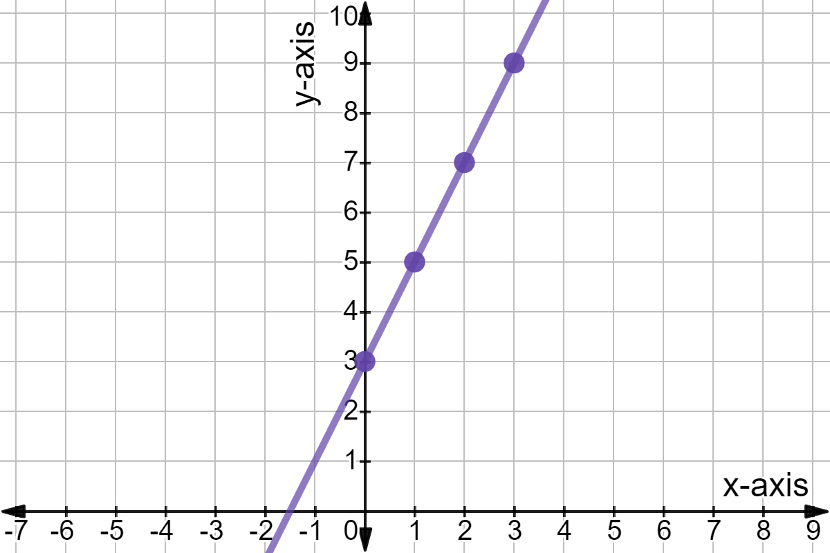
Which of the following is the input table for the function: f(x)=2x+3f(x)=2x+3

Choose one answer

Illustrated · 1 min

Graphing Linear Functions

Linear functions are basically functions made of straight lines! We'll see this concept a lot of algebra, so it's important to get a solid understanding of linear functions.

graphing linear functions
"linear" = line
characteristics of lines:
>slope
>$(x,y)$ coordinates
>$y$-intercept
>$x$-intercept
forms of linear equations:
>point slope form $y-y_1=m(x-x_1)$
>standard form $ax+by=c$
>slope-intercept form $y=mx+b$

Image source: by Anusha Rahman

Linear functions are different from non-linear functions, like quadratic or cubic functions. Linear functions have xx values. Quadratic functions use x2x^2, and cubic functions x3x^3. You'll learn about these two later!

Type a concept, like “slope” or “photosynthesis”.

↑ ↓ to choose · Enter to openSearch explanations and problems