Графіки увігнутих функцій

Before Diving In

Now that we've covered extrema, let's move on to a more complex topic.

Before diving into this lesson, you may want to review how to find the derivative of a function, using a derivative test, and using integrals. If you haven't covered these topics yet, no worries! You have plenty of time before you will learn this complicated stuff.

Riemann Sums and Convexity

In this explanation, we're going to unite the concepts of Riemann Sums and Convexity. The reason we do this is because convexity helps us understand how powerful Riemann Sums are. But we're not going to assume knowledge of anything about Riemann Sums, so let's begin with some definitions, and we'll talk about convexity later.

A Riemann Sum is an approximation of an integral based on evaluating the function you're integrating at particular points.

There are different types of Riemann Sums but constructing any of them follows roughly the same pattern:

i) Pick an interval over which you're integrating your function

ii) Break that interval into (equally-sized) sub-intervals; for example, we can break $[0, 4]$ into $[0, 1], [1, 2], [2, 3],$ and $[3, 4].$

iii) Make a rectangle with one side on the x-axis and the opposite parallel to the x-axis, while the other two sides are parallel to the y-axis. The height of this rectangle will be determined on which type of Riemann Sum we use, so we'll get back to this later. The widths of the rectangles are the intervals we constructed in part ii).

iv) Calculate the areas of all the rectangles made in step iii) and add them.

This answer will be our "guess" as to the value of the integral. Sometimes our guess is close, and sometimes it's not; it depends on certain characteristics of the function. It also, of course, depends, on which type of Riemann Sum we use, and how many rectangles we use.

I'm going to introduce all three types of Riemann Sums and do a bunch of calculations with the same function so we can compare how all three types of sums work.

I'm going to first talk about the Midpoint Riemann Sum. The Midpoint Riemann Sum is one for which we evaluate the function we're integrating at the midpoint of each interval, and use those values to determine the heights of the rectangles.

Our example function is going to be $f(x) = x^2 + 1,$ where we integrate over the interval $[0, 3].$ We also get to choose the sizes of the rectangles, so for now we'll have each one be $1$ unit, for a total of three rectangles.

The midpoints of our mini-intervals are $\frac{1}{2},$ $\frac{3}{2},$ and $\frac{5}{2}.$ This means our key step is to evaluate the function at these three points:

$$\begin{align} f\left(\frac{1}{2}\right) &= \left(\frac{1}{2}\right)^2 + 1 = \frac{5}{4} \\ f\left(\frac{3}{2}\right) &= \left(\frac{3}{2}\right)^2 + 1 = \frac{13}{4} \\ f\left(\frac{5}{2}\right) &= \left(\frac{5}{2}\right)^2 + 1 = \frac{29}{4}. \end{align}$$

Now, these are the heights of the three rectangles. We know they all have length $1$ because we know their "horizontal" side lengths are along the intervals $[0, 1],$ $[1, 2],$ and $[2, 3].$ Therefore, the total area is

$$\frac{5}{4} \cdot 1 + \frac{13}{4} \cdot 1 + \frac{29}{4} \cdot 1 = \frac{47}{4}.$$

Mentally take note of this value as we'll look to compare it to the values of the other Riemann Sums. Speaking of which, let's define them.

The Left Riemann Sum uses the left-endpoints of the mini-intervals we construct and evaluates the function at THOSE points to determine the heights of our rectangles. Let's calculate the Left Riemann Sum for the same function. The left endpoints of the intervals are $0, 1,$ and $2.$ So we evaluate $f$ there:

$$\begin{align} f(0) &= (0)^2 + 1 = 1 \\ f(1) &= (1)^2 + 1 = 2 \\ f(2) &= (2)^2 + 1 = 5. \end{align}$$

So the heights of our rectangles are $1, 2,$ and $5.$ The widths of the rectangles are still $1$ unit each because we didn't change our intervals. Then the area is

$$1 \cdot 1 + 2 \cdot 1 + 5 \cdot 1 = 8.$$

Finally, the Right Riemann Sum uses the right-endpoints of the mini-intervals we construct and evaluates the function at THOSE points to determine the heights of our rectangles. For our particular example, the right endpoints are $1, 2,$ and $3.$ We already computed $f(1)$ and $f(2),$ while $f(3) = 3^2 + 1 = 10.$ Then the total area is

$$2 \cdot 1 + 5 \cdot 1 + 10 \cdot 1 = 17.$$

So in summary, the Left Riemann Sum has value $8,$ the Middle Riemann Sum has value $\frac{47}{4},$ and the Right Riemann Sum has value $17.$

Congratulations! You've now computed some simple Riemann Sums, of each of the three main types we want to talk about here. But this leaves a few questions unanswered.

The first is, why do we care about Riemann Sums? Couldn't we just have easily calculated

$$\int^{3}_{0}(x^2 + 1)dx?$$

Well in this case, yes, but let's say you instead are asked to integrate

$$\int^{-44}_{17}xe^{x^2 + x}\arctan(x^2 - 2) + 3dx.$$

Yikes! That's not going to be fun. And I doubt it's possible to compute exactly. But you can use the same Riemann Integral Technique to get an ESTIMATE of what the value is. Oftentimes in industry an exact value isn't necessary, and an approximation is enough, so one can do a calculation like the ones we just showed you. It's also worth noting that especially if you have big numbers or a lot of rectangles, these calculations are usually done on a computer.

Here's another question you might think about: how many rectangles do we need? We can use as many as we want, but as we add more, the widths of them will be smaller, and we will have to sum more areas. If we get to using so many, we will get very close to the exact value of the integral. This is exactly why we care about limits, and it so turns out that the integral will equal the exact same thing as any of the Riemann Sums if we approach infinitely many rectangles (and of course, the individual area of each rectangle will go to zero, but we gain more and more rectangles, so these effects essentially cancel each other out).

If you're looking for a big fancy formula, you won't have to use one in practice for this, but it's helpful for understanding what's going on. Here's a formula for using Left Riemann Sums to find the value of the integral for a function $f:$

$$\int^{b}_{a}f(x)dx = \lim_{n \rightarrow \infty}\sum^{n - 1}_{k = 0}\frac{b - a}{n} \cdot f\left(a \cdot \frac{k}{n} + b \cdot \frac{n - k}{n}\right)$$

The important things are this: $b - a$ is the total length of the interval you're integrating over, and we evaluate $f$ at the beginning of each mini-interval. The exact locations are determined as a weighted average between the two endpoints of the big interval, $a$ and $b.$

The last thing I want to talk about is how good our approximations are. That is, how close can we get to the actual value of an integral using a Riemann Sum? There are so many functions that it ultimately depends. I'm going to explore this from two different dimensions.

The first goes back to the formula we just talked about:

$$\int^{b}_{a}f(x)dx = \lim_{n \rightarrow \infty}\sum^{n - 1}_{k = 0}\frac{b - a}{n} \cdot f\left(a \cdot \frac{k}{n} + b \cdot \frac{n - k}{n}\right)$$

Well, there is a near-identical one for the Right Riemann Sum:

$$\int^{b}_{a}f(x)dx = \lim_{n \rightarrow \infty}\sum^{n}_{k = 1}\frac{b - a}{n} \cdot f\left(a \cdot \frac{k}{n} + b \cdot \frac{n - k}{n}\right)$$

Both formulas involve limits, which eventually equal the same value: $\int^{b}_{a}f(x)dx.$ But the expressions inside the limits are different, so what gives?

What this means we should expect is that, as we get closer to the exact value of $\int^{b}_{a}f(x)dx,$ the values of the Riemann sums we use to estimate this value should get close to EACH OTHER. If two Riemann sums have values close to that of $\int^{b}_{a}f(x)dx,$ then their values are close to each other as well. How close?

We do a quick calculation to help answer this question. Pick a large $n,$ representing a Riemann Sum with many rectangles. Then we ask about the difference between the values of the Left and Right Riemann Sums. The formulas for the Left and the Right Riemann Sums are

$$L = \sum^{n - 1}_{k = 0}\frac{b - a}{n} \cdot f\left(a \cdot \frac{k}{n} + b \cdot \frac{n - k}{n}\right)$$ $$R = \sum^{n}_{k = 1}\frac{b - a}{n} \cdot f\left(a \cdot \frac{k}{n} + b \cdot \frac{n - k}{n}\right)$$

and to get them we just pull the expressions out of the limits from the formulas for the exact value of the integral $\int^{b}_{a}f(x)dx.$ To find how the two estimates of this integral differ, we subtract one from the other and take an absolute value (think of the difference as a distance, perhaps between two points on the number line; distances are always regarded as nonnegative numbers by convention). So we define this distance to be $|L - R|,$ and we plug in the values of $L$ and $R$ to get

$$\left|\sum^{n - 1}_{k = 0}\frac{b - a}{n} \cdot f\left(a \cdot \frac{k}{n} + b \cdot \frac{n - k}{n}\right) - \sum^{n}_{k = 1}\frac{b - a}{n} \cdot f\left(a \cdot \frac{k}{n} + b \cdot \frac{n - k}{n}\right)\right|$$

What do we do now? Well this is something called a telescoping series, because most of the terms cancel out between the two sums. The only terms that are left are

$$\left|\frac{b - a}{n}f(0) - \frac{b - a}{n}f(n)\right| = \frac{b - a}{n}\left|f(a) - f(b)\right|.$$

If $n$ is large, then this number is going to be quite small. It says that if $n$ is large, the Left and Right Riemann Sums have almost the same value.

Finally, I want to do another calculation that is specific to when we integrate convex functions. A convex function is one defined so that for any $x, y \in \mathbb{R}$ and any $\lambda \in [0, 1],$

$$f(\lambda x + (1 - \lambda) y) \leq \lambda f(x) + (1 - \lambda) f(y).$$

Colloquially, convex functions curve upward. $e^x,$ $x^2,$ $x,$ and $x^4$ are examples of convex functions. They are plentiful and worth investigating a bit more in detail. We're going to show a nice inequality is true if $f$ is a convex function. Again we state the formula for the Right Riemann Sum used to estimate $\int^{b}_{a}f(x)dx.$

$$R = \sum^{n}_{k = 1}\frac{b - a}{n} \cdot f\left(a \cdot \frac{k}{n} + b \cdot \frac{n - k}{n}\right)$$

Notice that $\frac{k}{n}$ and $\frac{n - k}{n}$ are both between $0$ and $1$ because $k$ and $n$ are positive and $n \geq k.$ This means if $f$ is convex we can do the following for each $k$ in the sum:

$$f\left(a \cdot \frac{k}{n} + b \cdot \frac{n - k}{n}\right) \leq \frac{k}{n}f(a) + \frac{n - k}{n}f(b)$$

Essentially we're using the definition of convexity where $\lambda = \frac{n}{k},$ $x = a,$ and $y = b.$

Now it's time for some algebra. Multiply both sides by $\frac{b - a}{n},$ which is also positive.

$$\frac{b - a}{n} f\left(a \cdot \frac{k}{n} + b \cdot \frac{n - k}{n}\right) \leq \frac{k(b - a)}{n^2}f(a) + \frac{(n - k)(b - a)}{n^2}f(b)$$

Now we sum both sides of this inequality over all $k$ between $1$ and $n.$ The lesser side is just the definition of $R,$ so

$$R \leq \sum^{n}_{k = 1}\left(\frac{k(b - a)}{n^2}f(a) + \frac{(n - k)(b - a)}{n^2}f(b)\right).$$

Why is this helpful? Well, notice both terms in the sum have factors that don't depend on $k:$

$$R \leq \frac{b - a}{n^2}f(a)\sum^{n}_{k = 1}k + \frac{b - a}{n^2}f(b)\sum^{n}_{k = 1}(n - k).$$

If we evaluate both of the sums left, we get

$$R \leq \frac{b - a}{n^2}f(a) \cdot \frac{n^2 + n}{2} + \frac{b - a}{n^2}f(b) \cdot \frac{n^2 - n}{2}.$$

Finally, we can factor and cancel out some factors of $n:$

$$R \leq \frac{b - a}{n}\left(\frac{f(a)(n + 1)}{2} + \frac{f(b)(n - 1)}{2}\right).$$

Why is this helpful? Well, if we don't care about the exact value of the Riemann Sum and an estimate is good enough for us, this expression only involves evaluating $f$ twice, even if there were a lot of rectangles. In some sense, we are giving up some accuracy to save a lot of time.

In summary, if a math problem is hard, look for clever ways to make it easier. Once you unlock the tools of calculus it becomes more apparent how you can do this.

In this explanation I'm going to talk about concavity and convexity using mostly graphs. "Concavity" and "convexity" are both often used as qualitative descriptions of the shape of a graph.

In short, a concave (or concave down) function is one whose graph is shaped like an upside-down U, or that decreases in value "faster and faster."

As you might have guessed, then, a convex (or concave up) function is one whose graph is shaped like a right-side up U, or that increases in value "faster and faster."

Before, I show any actual graphs, let me share a little trick my high school math teacher taught me to distinguish the terms "convex" and "concave." He said that the "concave" graph is the one that is shaped like the roof of a cave, just like the picture below.

Then, by process of elimination, the other "type" of graph is the convex one.

Since I described these graphs as right-side up and upside-down "U"s, let's look at the classic U-shaped graphs, the parabolas $f(x) = x^2$ and $g(x) = -x^2.$

The red graph, $f(x) = x^2,$ is convex, while the blue graph, $g(x) = -x^2,$ is concave. This suggests an important relationship between convex and concave graphs:

If $f$ is convex, then $-f$ is concave, and vice-versa.

That is, we can flip between a convex graph and a concave graph by changing its sign.

Another thing to note is related to the tangent line at the inflection point. If the entirety of the graph lies below the tangent line, then we say that the graph is concave. The opposite is true for convex graphs. The the entirety of the function lies above the tangent line, we say that the graph is convex.

Here's another pair of graphs that illustrates a different property of convex/concave graphs.

In this case, $f(x) = x^2$ and $g(x) = x^2 + 2,$ which are the same after a vertical translation. Despite doing such a translation, the graphs have the same overall shape, which suggests another fact:

If we translate a concave graph horizontally or vertically, it is still concave. If we translate a convex graph horizontally or vertically, it is still convex.

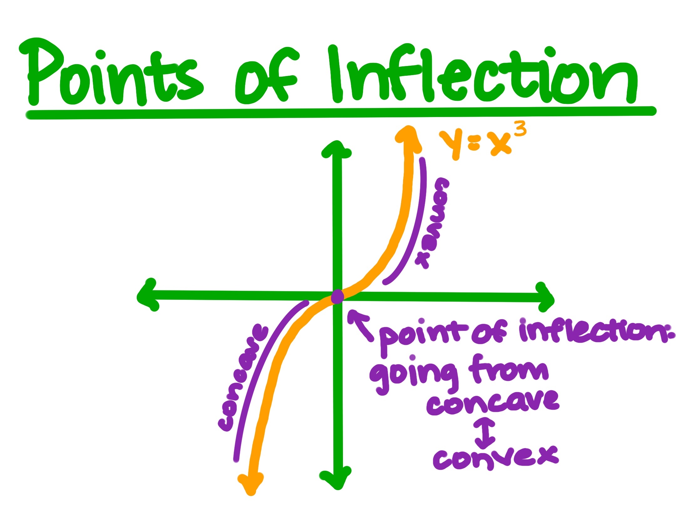
Here's one more funky thing about concave and convex graphs: a graph can be concave on one part of its domain and convex on the other. If the graph switches between being convex and concave, the point(s) at which this happens are called inflection points.

The function $f(x) = x^3$ is a simple example of a function that changes between concave and convex. It is concave when $x < 0$ and convex when $x > 0.$ This means the [only] inflection point is at $x = 0.$

In this explanation we're going to talk about concavity and convexity from an algebraic standpoint, with inequalities.

A function $f$ is convex if for all $x$ and $y$ in the function's domain and any choice of number $\lambda \in [0, 1],$ the following inequality is true:

$$f(\lambda x + (1 - \lambda)y) \leq \lambda f(x) + (1 - \lambda) f(y).$$

On the other hand, a function $f$ is concave if for all $x$ and $y$ in the function's domain and any choice of number $\lambda \in [0, 1],$ the following inequality is true:

$$f(\lambda x + (1 - \lambda)y) \geq \lambda f(x) + (1 - \lambda) f(y).$$

In some cases we can split the function's domain and see it's concave on one portion of the domain and convex on another, but we'll get to that later. For now we provide some concrete examples of functions that are concave everywhere or convex everywhere.

Example: Let's think about the function $f(x) = x^2 + 1,$ whose domain is $\mathbb{R}$ (that is, a value of $f(x)$ exists for any real number $x$ we choose).

We will demonstrate that this function is convex. Here's how we do that: we pick any two real numbers $x$ and $y,$ as well as a parameter $0 \leq \lambda \leq 1.$ Then we show that the following inequality must be true:

$$f(\lambda x + (1 - \lambda)y) \leq \lambda f(x) + (1 - \lambda) f(y).$$

We know that $f(x) = x^2,$ so substituting this function definition means we need to actually show that THIS inequality is true:

$$(\lambda x + (1 - \lambda) y)^2 \leq \lambda x^2 + (1 - \lambda) y^2.$$

We're going to work backwards to show this is true; that is, we'll simplify this inequality until we get something which we KNOW is true. Let's begin by expanding the square on the left-hand side:

$$\lambda^2 x^2 + 2\lambda xy(1 - \lambda) + y^2(1 - \lambda)^2 \leq \lambda x^2 + y^2(1 - \lambda)$$

This is going to require some very careful factoring, and you may want to look over factoring by grouping before continuing on.

Now then, let's get to work. We are going to factor by grouping by moving everything to one side of the inequality. Start by subtracting $\lambda x^2 + y^2(1 - \lambda)^2$ from both sides:

$$2\lambda xy(1 - \lambda) \leq \lambda x^2 + y^2(1 - \lambda) - \lambda^2 x^2 + y^2(1 - \lambda)^2.$$

We can group the first and third terms, and the second and fourth terms, pulling out common factors:

$$2\lambda xy(1 - \lambda) \leq \lambda x^2(1 - \lambda) + y^2(1 - \lambda)(1 - (1 - \lambda)).$$

The greater side can be simplified:

$$2\lambda xy(1 - \lambda) \leq \lambda x^2(1 - \lambda) + y^2\lambda (1 - \lambda).$$

If $\lambda = 1$ then both sides of the inequality equal $0$ and we are done. The reason we think to check this is because EVERY term in the inequality shares a factor of $1 - \lambda,$ so we can just divide it away now (and moreover, $1 - \lambda$ will never be negative, so we don't even have to worry about flipping the inequality sign).

$$2\lambda xy \leq \lambda x^2 + y^2\lambda.$$

Now it becomes even more clear how to proceed. If $\lambda = 0,$ then both sides of the inequality equal $0,$ so let's rule out this case and keep going. Divide both sides of the inequality by $\lambda:$

$$2xy \leq x^2 + y^2.$$

We're almost done: subtract $2xy$ from both sides:

$$0 \leq x^2 - 2xy + y^2 = (x - y)^2,$$

which we know is true, so we're done! Huzzah!

Sadly, this approach does not provide much of a sense of why $f(x) = x^2$ is convex, if you just look at the algebra. A more verbal way of considering convexity is to see that the function $f(x)$ grows "faster and faster," and this can be verified if you graph $f(x) = x^2$ by hand or with a calculator.

Now let's do an example of showing that a function is concave. The procedure, algebraically speaking, is very similar to showing that a function is convex. We're trying to show the same inequality as before, just with the inequality sign flipped around. As you might expect, a concave function is one that can be interpreted to be growing "slower and slower."

What is the first example of such a function you thought of? Odds are it was the square root function

$$g(x) = \sqrt{x}.$$

For our second example we will show that $g(x)$ is concave using the definition we gave at the beginning, making this intuition something mathematically more meaningful (say that three times fast). Unlike the last example, this time our domain is the nonnegative numbers, because a square root is only defined for nonnegative numbers.

Let's let $x$ and $y$ be nonnegative real numbers, and have $\lambda$ be a parameter (a number) between $0$ and $1$ inclusive. Then our goal is to show that

$$g(\lambda x + (1 - \lambda)y) \geq \lambda g(x) + (1 - \lambda)g(y).$$

Substitute the function $g(x) = \sqrt{x}$ in here:

$$\sqrt{\lambda x + (1 - \lambda)y} \geq \lambda \sqrt{x} + (1 - \lambda)\sqrt{y}.$$

The best way to get rid of all the square roots is to square both sides of the inequality (both sides are nonnegative, so no need to flip the inequality sign):

$$\lambda x + (1 - \lambda)y \geq \lambda^2 x + 2\lambda \sqrt{xy} (1 - \lambda) + (1 - \lambda)^2 y.$$

Much like in the first example, we're going to do some rearranging to exploit common factors. Subtract $\lambda^2 x$ from both sides:

$$\lambda x - \lambda^2 x + (1 - \lambda)y \geq 2\lambda \sqrt{xy} (1 - \lambda) + (1 - \lambda)^2 y.$$

The first two terms on the left-hand side share a factor of $\lambda x,$ so let's factor that out:

$$\lambda x(1 - \lambda) + (1 - \lambda)y \geq 2\lambda \sqrt{xy} (1 - \lambda) + (1 - \lambda)^2 y.$$

In a similar mindset, subtract $(1 - \lambda)^2 y$ from both sides:

$$\lambda x(1 - \lambda) + (1 - \lambda)y - (1 - \lambda)^2y \geq 2\lambda \sqrt{xy} (1 - \lambda).$$

Now, the last two terms on the left-hand side share a factor of $(1 - \lambda)y,$ so let's pull that out:

$$\lambda x(1 - \lambda) + (1 - \lambda)y(1 - (1 - \lambda)) \geq 2\lambda \sqrt{xy} (1 - \lambda).$$

The expression $(1 - (1 - \lambda))$ just simplifies to $\lambda,$ so

$$\lambda x(1 - \lambda) + \lambda y(1 - \lambda) \geq 2\lambda \sqrt{xy} (1 - \lambda).$$

Now we have a bunch of common factors that have "magically" appeared in ALL the terms. To exploit this, notice that if $\lambda = 0$ or $\lambda = 1,$ both sides of the inequality just turn into $0.$ Otherwise, we can divide both sides by $\lambda(1 - \lambda)$ (which is nonnegative, so no need to flip the inequality sign):

$$x + y \geq 2\sqrt{xy}$$

The fact that all the $\lambda$s are gone is a sign we are almost done! Just subtract $2\sqrt{xy}$ from both sides:

$$x - 2\sqrt{xy} + y \geq 0.$$

Now the left-hand side is just a perfect square in disguise, and in fact we have

$$(\sqrt{x} - \sqrt{y})^2 \geq 0,$$

which is true since the square of anything (real) is nonnegative. Therefore, $g$ is a concave function on its domain $[0, \infty).$

As a parting party trick, here's one other handy fact:

-If $f(x)$ is a convex function, then $-f(x)$ is a concave function.

-If $g(x)$ is a concave function, then $-g(x)$ is a convex function.

Well, I guess that was two handy facts. Anyway, it means that it you flip the graph of a function upside down, its concavity changes. From this, and the examples we did, we can conclude that $-x^2$ is concave, whereas $-\sqrt{x}$ is convex.

Concavity is a topic that you'll delve into deeper in calculus. For now, here's a simple understanding of what it is.

Concavity and Concave Functions

A function is concave (or concave down) when its curve resembles a hump, like the graph above. The way I was taught was it's concave because it resembles a cave. There's two side walls and a top to it.

Convexity and Convex Functions

A function is convex (or concave up) when its curve resembles a $U$ like the graph above. The way I think about it is you have two walls next to you and if you look up you'll see the sky and not the roof of a cave, so therefore its convex.

Both

A graph can be both concave and convex, even switching multiple times at different parts. Be careful, though, on no portion of the graph will the function be both concave and convex, only one or the other.

Above is a graph of a cubic polynomial. The function is concave up until the middle point, where it switches to convex. The point in which a graph switches from one concavity to another is called an inflection point.

(Video) Finding Concavity and Points of Inflection Graphically

by Anusha Rahman

In this lesson by Anusha Rahman, you will learn how to find points of inflection and concavity graphically.

Summary

With a concave graph the graph opens downward or is shaped like a cave. Some people also call this type of shape, concave down.

A convex graph opens upward or is shaped like a cup. Some people also call this shape concave up.

A point of inflection is where the function changes direction. Qualitatively, we can find this point by looking at the graph. Quantitatively, we can use the second derivative.

Points of Inflection

Points of inflection are the points at which the graph goes from concave to convex, or vice versa. This relates to functions increasing and decreasing.