Асиметричні графіки

Visualizing Skew Using a Graph

The skewness of a graph is simply a way of describing the shape of a distribution. Before explaining some of the details, we can gain a visual intuition for what skew is:

So, when looking at a graph of the distribution, see which side of the graph has more of a "tail", and that will be the direction of the skew. The "tail" side is longer! This might seem a little weird, since the left skew graph seems to be leaning to the right and vice versa for the right skew graph. Remember that skew refers to where the tail of the graph is, not where datapoints are.

Note: Left skew is also known as negative skew and right skew is also known as positive skew. Keep this in mind if you read stuff online about skew.

Understanding What a Tail Is

A "tail" of a graph is a very visual concept. Essentially, a tail refers to the part of a graph of a distribution which tapers off on one side.

Looking back at the graphs from above, we can see that the graph on the right has a long section (from around $1$ onwards) where the graph tapers off. This is what we refer to as a tail. So for the graph on the right, the tail is on the right.

Looking at the leftmost graph, we see the graph tapers off to the left (starting at around $-1$).

See below for the same graphs but with the tails of the left and right graphs circled in

Effects of Skew on Measures of Central Tendency

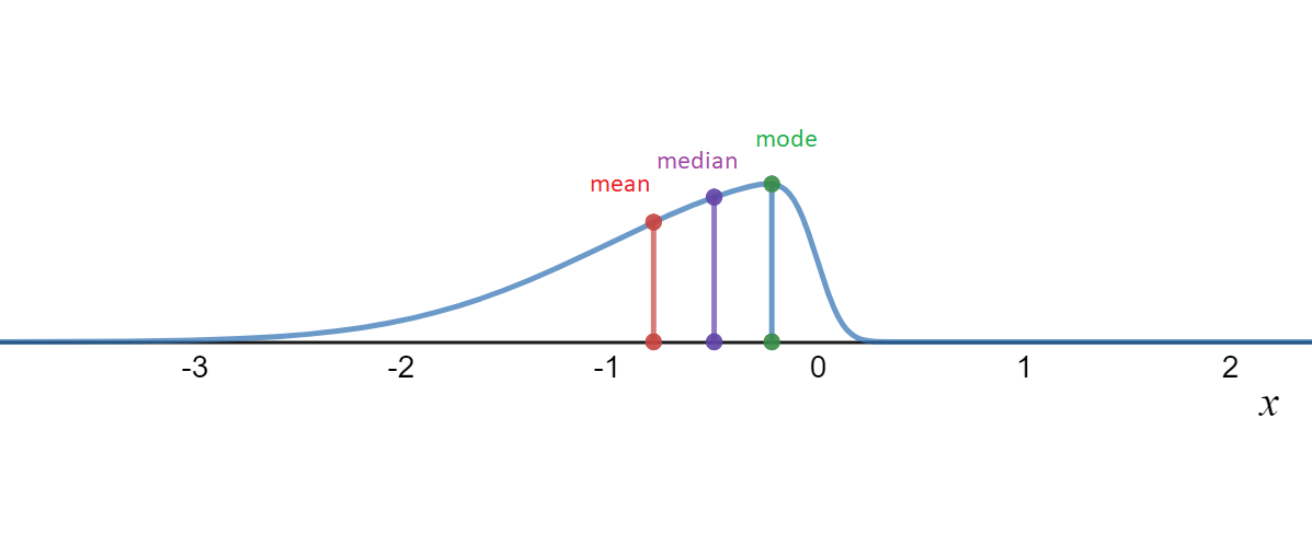
Now, let's use our Measures of Central Tendency and plot the mean, median, and mode of graphs which have left or right skew.

You may have noticed in the graph that when there is left skew, the mean is to the left of the median/mode while with right skew, the mean is to the right of the median/mode. This will almost always be true of left and right skewed graphs.

If you're curious about cases where these rules don't work, try checking out the Binomial Distribution. For some values, the binomial distribution has the same mean, median, and mode but still has left skew!

There is a more specific way to measure how skewed a distribution is, called Pearson's moment coefficient of skewness, but it is quite advanced. For now, focus on finding the tail of the distribution. If there is no information on where the tail of the distribution is, try using the mean, median, and mode to determine skew.

Visualizing Skew with Box and Whisker Plots

Another common way of visualizing distributions is Box and Whisker Plots. As mentioned earlier, we can use multiple ways to measure the skew of a distribution. One way to do so is using Quartiles. We can say a distribution is left skewed if $Q2-Q1 > Q3-Q2$ while a distribution is right skewed if $Q2-Q1<Q3-Q2$.

This might not make much sense with a bunch of variables, so we can demonstrate it visually using box plots:

Now, $Q2-Q1$ is the size of the left rectangle while $Q3-Q2$ is the size of the right rectangle. In this case, we would say the distribution is left skewed.

A good way of remembering this rule is that a distribution is left skewed if the left rectangle is bigger than the right while the distribution is right skewed if the right rectangle is bigger than the left.

Sometimes, box plots are made vertically. In this case, right skew corresponds to the upper rectangle being bigger while left skew corresponds to the bottom rectangle being bigger.

Now, a natural thing to wonder is if all these ways of measuring skew are the same. If the box plot looks left skewed, then the mean might be less than the median/mode... Think about this for a little while then continue.

The answer is no! We can see this by looking at the data $[1,2,4,4,5,8]$. The mean of this data is $4$, the median is $4$ and the mode is $4$ (try to verify this yourself!). Now, let's look at the box plot:

Notice that the left rectangle is bigger than the right triangle. So this indicates left skew. However, we already saw that the mean, median, and mode are all the same, which indicates no skew! This is very important since it shows that the way we measure skew determines if a distribution is skewed or not.

Summary

In general, here are some rules for determining the skew of a distribution:

• If you get a graph of a distribution, look for the tail of the graph to determine skew.

• If you get a box plot, look for which rectangle is bigger to determine skew.

• If you have only the data, try making a box plot/graph and using that to determine skew.

• If none of these methods are working, compare the mean, median, and mode to determine skew.

Skewed Graphs

"Skew" is basically a descriptor of distributions. Instead of being symmetric (think bell curve or normal distributions), skewed graphs are usually shifted to one side. The other side consists of a trailing tail.

The way to analyze a skewed graph is to see where the mean lies in relation to the median. Take the AMC score distribution-- since it is right-skewed, that denotes the mean (average) will be higher than the median (middle) score. That is because the scores from 120 to 150 are pulling the average up toward positive infinity, while most students scored from 40 to 80. In fact, the reported median was 58.5 while the reported mean score was 63.34.

Here's what a left-skewed graph looks like:

Notice that in the left-skewed graph, the mean (red) is numerically less than the median (purple). This is similar to the example above, but those few extremely negative values pull the mean down toward negative infinity.

In conclusion, a quick way to remember how to differentiate between a right and left skewed distribution is 'few is skew'. The side with fewer values (look for the trailing tail) is the skew.

Skewed Graphs

In statistics, you've seen normally distributed graphs, such as the one below.

This is the most common type of statistical model. Note that the mean and the median are the same value in normal distributions.

However, we will not always have a nice, neat, symmetrical distribution like this. Sometimes, the graph will seem to skew left or right, meaning that it is asymmetric and it has a tail in one of the two directions. Let's take a look at some examples of what left and right skewed graphs may look like.

Left-Skewed Graphs

The graph above is an example of a left-skewed graph. It is left-skew because the tail of the graph is toward the left.

Left-skewed distributions are also referred to as "negatively-skewed" distributions. That is because the tail is in the negative direction of the number line (pointing leftward, past the point $0$ on the number line).

Notice the location of the mean and median in left-skewed distributions. You can tell this is a left-skewed distribution based on the location of the mean, which is to the left of the median. Since it is to the left, the value of the mean is less than the median.

Right-Skewed Graphs

The graph above is an example of a right-skewed graph. Like the left-skewed, you may have originally thought that the location of the bubble is what determines left vs. right, but it is in fact the tail that is the determinant.

Right-skewed distributions are also referred to as "positively-skewed" distributions since the tail is in the positive direction of the number line.

Notice the location of the mean and median in right-skewed distributions. You can tell this is a right-skewed distribution based on the location of the mean, which is to the right of the median. Since it is to the right, the value of the mean is more than the median. By this reasoning you should see that no graph can be both left and right-skewed.

What is skewness and what does it look like to be skewed?

Skewness is asymmetry in a statistical distribution, in which the curve appears to lean either to the left or to the right.

---

Note: Left skew is also sometimes referred to as being negatively skewed (because its tail trails in the negative direction), and right skew is sometimes referred to as being positively skewed.

---

Skewness can be quantified to define the extent to which a distribution is different than a normal distribution (bell curve). This is important because certain statistical methods can be used for a normal distribution but not skewed distributions or distributions with small sample sizes. Other statistical approximation methods can be used in these cases.

In a normal distribution, the graph appears as a classical, symmetrical "bell-shaped curve." This means that the mean/average of the data set and the mode are equal. Graphically, the mean and mode are located at the tallest point on the normal distribution.

---

Tip: To help remember what right and left skew distributions look like, remember that whatever the direction of the tail is trailing, that is the type of skewness it has.

---

Skewness looks different depending on what statistical graph we are using to help interpret the data.

Below is an example of left/right skewness with a Box-and-Whisker Plot

(Video) Skewness | Statistics

by Don't Memorise

As we previously learned about the normal distribution, the bell curve is centered at the mean and is symmetrical. However, normal distributions can become skewed, no longer being symmetrical. Watch this video by Don't Memorise to learn more!

Normal distributions can be skewed when the mean is not located in the center of the distribution. Instead it is located to the side.

When the mean is toward the side, a tail, a slight tapering of the curve, forms on the other side. If the tail is on the positive/right side, then we say the distribution is positively skewed or skewed to the right. If the tail is on the negative/left side, then we say the distribution is negatively skewed or skewed to the left.