近似与黎曼和

Video · + 2 min read

(Video) Approximating Definite Integrals Using Rectangles

by PatrickJMT

Here's a video by patrickJMT where he shows you how to approximate a definite integral using rectangles.

It is important to know that there are three types of rectangles we can take when approximating: left, right, and midpoint. As you will see in the following examples, they do give different results.

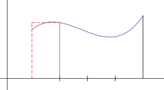
The left rectangle approximation is when you make the left hand points of the pieces the height of the rectangles.

Build a rectangle where the top left intersects the curve

The right rectangle approximation is when you make the right hand points of the pieces the height of the rectangles.

Build a rectangle where the top right intersects the curve

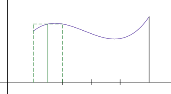
Finally, a midpoint rectangle approximation is when you make the midpoints of the pieces the height of the rectangles.

Build a rectangle where the midpoint intersects the curve, and the left and right top corners need not hit the curve

The first problem he looks at is:

Approximate ∫02(16−x2)dx\int_0^2(16-x^2)dx using n=4n=4 rectangles and left endpoints.

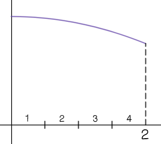
To start, we should draw the graph on the interval [0,2][0,2].

just draw the graph on the interval [0, 2], ignore the rest of it for now

Next, it tells us to use n=4n=4 rectangles. To determine the spacing we can use the formula: Δx=b−anΔx=2−04=12\begin{align} \Delta x&=\frac{b-a}{n}\\ \Delta x&=\frac{2-0}{4}\\ &=\frac12 \end{align}

Label the x-axis in 1/2-unit increments

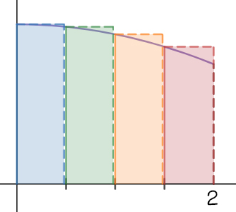
Finally, it wants the rectangles to be left endpoints. This means the rectangles' height is based off the left point.

Draw rectangles within each 1/2-unit interval with the top left corner intersecting the curve

Left Endpoints

Finally we just sum up the area of each rectangle. A≈R1+R2+R3+R4A≈0.5f(0)+0.5f(0.5)+0.5f(1)+0.5f(1.5)A≈0.5[f(0)+f(0.5)+f(1)+f(1.5)]A≈0.5[(16−02)+(16−0.52)+(16−12)+(16−1.52)]A≈0.5[16+15.75+15+13.75]A≈30.25\begin{align} A&\approx\color{blue}{R_1}+\color{green}{R_2}+\color{orange}{R_3}+\color{red}{R_4}\\ A&\approx\color{blue}{0.5f(0)}+\color{green}{0.5f(0.5)}+\color{orange}{0.5f(1)}+\color{red}{0.5f(1.5)}\\ A&\approx0.5[\color{blue}{f(0)}+\color{green}{f(0.5)}+\color{orange}{f(1)}+\color{red}{f(1.5)}]\\ A&\approx0.5[\color{blue}{(16-0^2)}+\color{green}{(16-0.5^2)}+\color{orange}{(16-1^2)}+\color{red}{(16-1.5^2)}]\\ A&\approx0.5[\color{blue}{16}+\color{green}{15.75}+\color{orange}{15}+\color{red}{13.75}]\\ A&\approx30.25 \end{align}

Because our rectangles are containing area above the curve, we know that our answer is an overestimate.

This part is not in the video but let's see what happens when we use right endpoints.

Approximate ∫02(16−x2)dx\int_0^2(16-x^2)dx using n=4n=4 rectangles and right endpoints.

Since everything else is staying the same, the graph and the pieces will be the same as before.

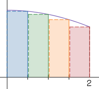
Draw rectangles within each 1/2-unit interval with the top right corner intersecting the curve

Right Endpoints

Because these rectangles leave out some area under the graph, we expect this approximation to be less than the one above. A≈R1+R2+R3+R4A≈0.5f(0.5)+0.5f(1)+0.5f(1.5)+0.5f(2)A≈0.5[f(0.5)+f(1)+f(1.5)+f(2)]A≈0.5[(16−0.52)+(16−12)+(16−1.52)+(16−22)]A≈0.5[15.75+15+13.75+12]A≈28.25\begin{align} A&\approx\color{blue}{R_1}+\color{green}{R_2}+\color{orange}{R_3}+\color{red}{R_4}\\ A&\approx\color{blue}{0.5f(0.5)}+\color{green}{0.5f(1)}+\color{orange}{0.5f(1.5)}+\color{red}{0.5f(2)}\\ A&\approx0.5[\color{blue}{f(0.5)}+\color{green}{f(1)}+\color{orange}{f(1.5)}+\color{red}{f(2)}]\\ A&\approx0.5[\color{blue}{(16-0.5^2)}+\color{green}{(16-1^2)}+\color{orange}{(16-1.5^2)}+\color{red}{(16-2^2)}]\\ A&\approx0.5[\color{blue}{15.75}+\color{green}{15}+\color{orange}{13.75}+\color{red}{12}]\\ A&\approx28.25 \end{align}

Now let's take the same problem but use the midpoints. Do you expect this approximation to be the most accurate?

Approximate ∫02(16−x2)dx\int_0^2(16-x^2)dx using n=4n=4 rectangles and right endpoints.

Draw rectangles within each 1/2-unit interval with the midpoint of the top of the rectangle intersecting the curve

Midpoints

The left side is missing area under the curve but the right side has area above the curve. Because of this, we expect the two to balance each other, giving us an approximation somewhere in-between the left endpoint and right endpoint. A≈R1+R2+R3+R4A≈0.5f(0.25)+0.5f(0.75)+0.5f(1.25)+0.5f(1.75)A≈0.5[f(0.25)+f(0.75)+f(1.25)+f(1.75)]A≈0.5[(16−0.252)+(16−0.752)+(16−1.252)+(16−1.752)]A≈0.5[15.9375+15.4375+14.4375+12.9375]A≈29.375\begin{align} A&\approx\color{blue}{R_1}+\color{green}{R_2}+\color{orange}{R_3}+\color{red}{R_4}\\ A&\approx\color{blue}{0.5f(0.25)}+\color{green}{0.5f(0.75)}+\color{orange}{0.5f(1.25)}+\color{red}{0.5f(1.75)}\\ A&\approx0.5[\color{blue}{f(0.25)}+\color{green}{f(0.75)}+\color{orange}{f(1.25)}+\color{red}{f(1.75)}]\\ A&\approx0.5[\color{blue}{(16-0.25^2)}+\color{green}{(16-0.75^2)}+\color{orange}{(16-1.25^2)}+\color{red}{(16-1.75^2)}]\\ A&\approx0.5[\color{blue}{15.9375}+\color{green}{15.4375}+\color{orange}{14.4375}+\color{red}{12.9375}]\\ A&\approx29.375 \end{align}

Accuracy

The smaller the error, the better the approximation of the actual value of the integral (which can't always be computed explicitly) TypeValueErrorAccuracyActual29.3ˉLeft30.250.916ˉ96.88%Right28.251.083ˉ96.31%Midpoint29.3750.0416ˉ99.86%\begin{array}{|c|c|c|c|} \hline \text{Type}&\text{Value}&\text{Error}&\text{Accuracy}\\ \hline \text{Actual}&29.\bar{3}&\\ \text{Left}&30.25&0.91\bar{6}&96.88\%\\ \text{Right}&28.25&1.08\bar{3}&96.31\%\\ \text{Midpoint}&29.375&0.041\bar{6}&99.86\%\\ \hline \end{array}

Type a concept, like “slope” or “photosynthesis”.

↑ ↓ to choose · Enter to openSearch explanations and problems