绘制二项式图像

Before this, know求多项式方程的根

Illustrated · 2 min

Now that we've covered the Intermediate Value Theorem, Descartes' Rule of Signs, and the Fundamental Theorem of Algebra, we can move to the last lesson.

End Behavior

The end behavior of a polynomial is how the ends of the functions behave. We want to see what happens to the graph of the function as xx approaches ∞\infty. In general, the function will either approach ∞\infty or −∞-\infty.

We can look at a graph and consider a polynomial's end behavior. Let's look at the graph of the parent function y=x3y=x^3.

Graph of y=x^3

Made using Desmos

From just looking at the graph, we can tell that as xx decreases, yy also decreases. We can write this mathematically as: x→−∞,y→−∞x \rightarrow -\infty, y \rightarrow -\infty. Similarly, as xx increases, yy also increases. Mathematically, this looks like: x→∞,y→∞x \rightarrow \infty, y \rightarrow \infty. These statements describe our end behavior.

When you learn calculus, you'll learn about limits and how you can use limits to determine end behavior. For now, we'll use graphing!

Graphing Polynomials Using Roots and End Behavior

Now that we've learned about end behavior, let's think about how we can use that to help us graph polynomials. If we are given a polynomial's roots and end behavior, we can create a sketch of what the graph looks like. The roots will tell us at which points the polynomial crosses the xx-axis. The end behavior will then fill in the rest of the information about the general shape of the polynomial.

Remember that this technique will give you a general idea of what a graphed polynomial looks like. This is by no means an exact method, but if you need to quickly understand the shape of a graph, then this method will help you!

Let's walk through an example.

Example

Say you're given the following information:

  • Roots: x=1x=1, x=2x=2

  • x→−∞,y→∞x \rightarrow -\infty, y \rightarrow \infty

  • x→∞,y→∞x \rightarrow \infty, y \rightarrow \infty

We know that our polynomial crosses the xx axis at two points because we have two roots. Our first thought may be that this polynomial is a quadratic, but that may not necessarily be the case. This polynomial could be a cubic function where one of the points of inflection is sitting on the xx-axis. For that reason, we will look at the end behavior before making a decision about the power of the polynomial.

The end behavior tells us that both ends of the function go upward, toward infinity. If this were a cubic function, one of the tails of the function would be going toward negative infinity, while the other would go toward positive infinity. For that reason, we can determine that this is a quadratic function.

So, we know that this polynomial is a quadratic with roots at x=1x=1 and x=2x=2, so now we can sketch the quadratic! We do not know the vertex of this quadratic, so we are missing some of the key characteristics, but we have a rough idea.
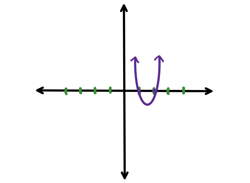
Sketch of a quadratic going through the points (1,0) and (2,0)

Image source: by Anusha Rahman

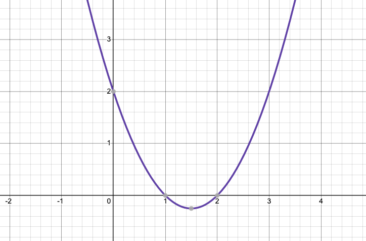
I can tell you that the polynomial is: y=x2−3x+2y=x^{2}-3x+2, and its graph looks like:

Graph of y=x^{2}-3x+2

Made using Desmos

Video · + 1 min read

(Video) Graphing Polynomial Functions Using End Behavior, Zeros, and Multiplicities

by Mario's Math Tutoring

In this video by Mario's Math Tutoring, you will learn how to graph polynomials with end behavior, zeroes, and multiplicity.

Summary

Example #1: Graph the polynomial, y=2(x−2)(x+3)(x−4)y=2(x-2)(x+3)(x-4).

##Zeroes

The first step is to find the xx-intercepts or zeroes. That is easy to do because this polynomial is already in factored form. The factors are: x=2x=2, x=−3x=-3, and x=4x=4.

Graph of zeroes, (-3,0), (4,0), and (2,0).

Made by desmos

##End-Behavior

Now that we have our xx-intercepts graphed, we can move on to step two, looking at the end-behavior of the polynomial. The end-behavior is what is happening at the ends of the graph. The leading coefficient will describe the end-behavior of the polynomial. If the leading coefficient is positive, the graph will go toward positive infinity. If the leading coefficient is negative, the graph will go toward negative infinity. To determine if the graph is going to the left or right, we will look at the degree of the polynomial. If the degree is odd, the left and right behavior will be opposite.

In our example, the leading coefficient is positive and has an odd degree.

##Multiplicity

Our third (and final) step is to look at the multiplicity. Multiplicity is looking at duplicates of zeroes. If there are no duplicates (odd multiplicity), the function will go straight through the xx-intercept (cross the xx-axis). If there is a duplicate, or a multiplicity of an even number, then the function will "bounce" off the xx-intercept (touch the xx-axis).

In our example, there are no multiples of the zeroes, so there is no "bouncing".

##Put it Together

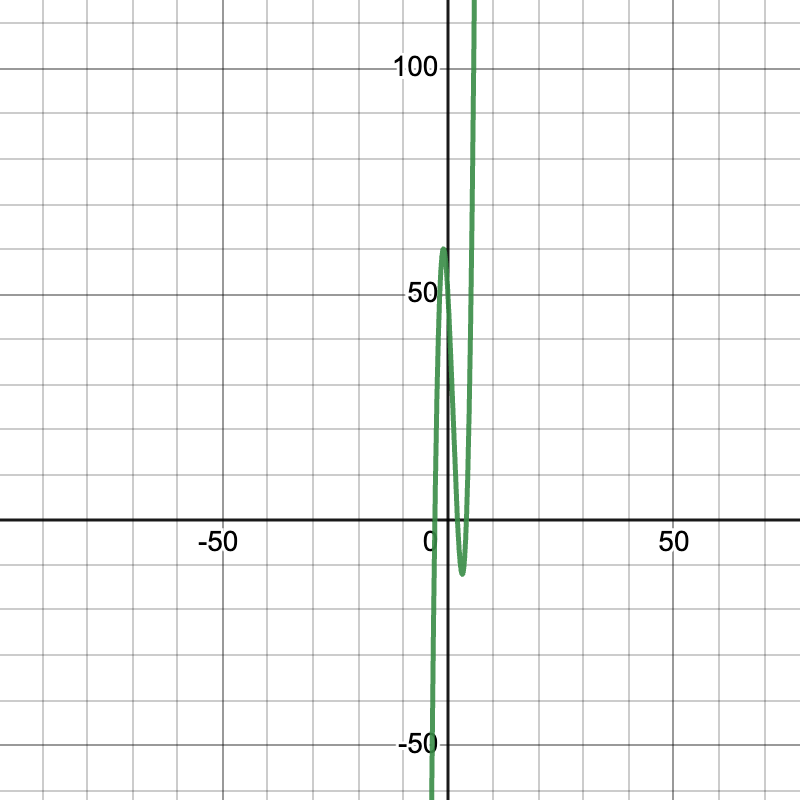
Putting it all together, we come up with the following graph! Here is the sketch of the graph:

Graph of y=2(x-2)(x+3)(x-4)

Made by demos

Mario has two more examples! Try them on your own, then watch the video to see if you're right!

Example #2: y=−x3+3x2y=-x^3 + 3x^2

Example #3: y=4(x+1)(x−3)2(x+2)3y=4(x+1)(x-3)^2(x+2)^3

Illustrated · 1 min

Graphing Polynomials: Using Roots and End Behavior

We've already learned about roots and end behavior with polynomials - we can now use those to graph polynomials. The roots are where the polynomial graph touches the xx-axis, AKA zeros.

The end behavior tells you what the graph does far to the left and to the right. To figure that out, look at the leading term (the one with the highest power of xx. If the degree is even and the leading coefficient is positive, both ends go up. If it's even and negative, both ends go down. If the degree is odd and the leading coefficient is positive, the left end goes down and the right end goes up.

Once you know the roots and the end behavior, you can make a pretty solid sketch of the graph. First plot the roots, decide how the graph moves at each root, and look at the end behavior. The xx-intercepts of a graph can be used to find or approximate zeros.

Graphing Polynomials: Roots + End Behavior
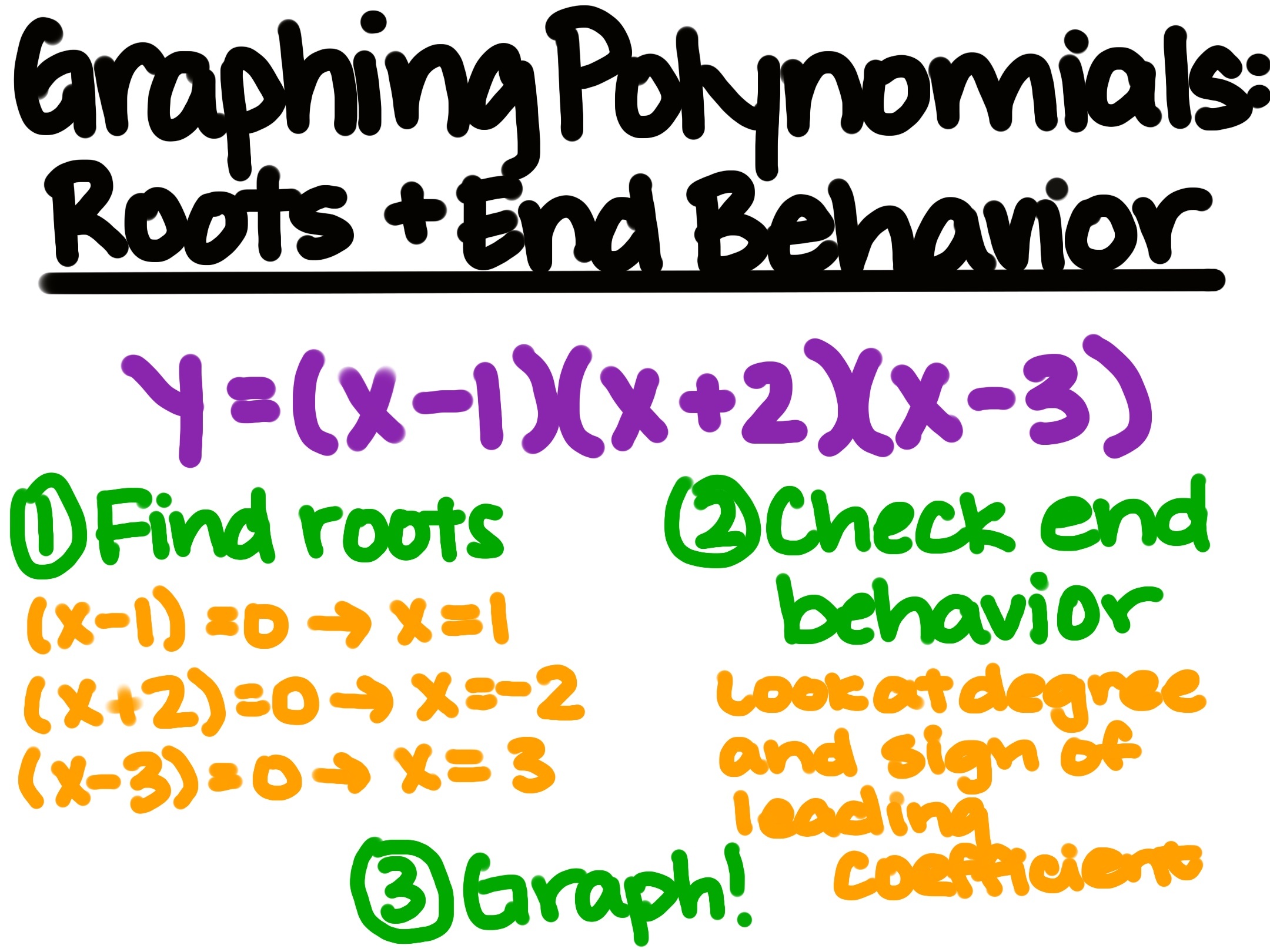
y = (x-1)(x+2)(x-3)
1) Find roots
(x-1) = 0 --> x=1 
(x+2) = --> x=-2
(x-3) = 0 --> x=3
2) Check end behavior
Look at degree and sign of leading coefficient
3) Graph

Image source: by Anusha Rahman

Let's dive deeper into the above polynomial.

y=(x−1)(x+2)(x−3)y=(x-1)(x+2)(x-3)

Step 1: Find the Roots

To find the roots, set y=0y=0:

  • (x−1)=0→x=1(x-1) = 0 \rightarrow x=1
  • (x+2)=0→x=−2(x+2) = 0 \rightarrow x=-2
  • (x−3)=0→x=3(x-3) = 0 \rightarrow x=3

So, the graph will cross the xx-axis at x=1,−2,3x=1, -2, 3.

Step 2: Check the end behavior

Since this is an odd-degree polynomial (degree is 33) and the leading coefficient is positive, we know that:

  • As x→−∞,f(x)→−∞x \rightarrow -\infty, f(x) \rightarrow -\infty, so the left end goes down
  • As x→∞,f(x)→−∞x \rightarrow \infty, f(x) \rightarrow -\infty, so the right end goes up

Step 3: Sketch the graph

Now that we know the roots and the end behavior, we can sketch the graph. Try it on your own!

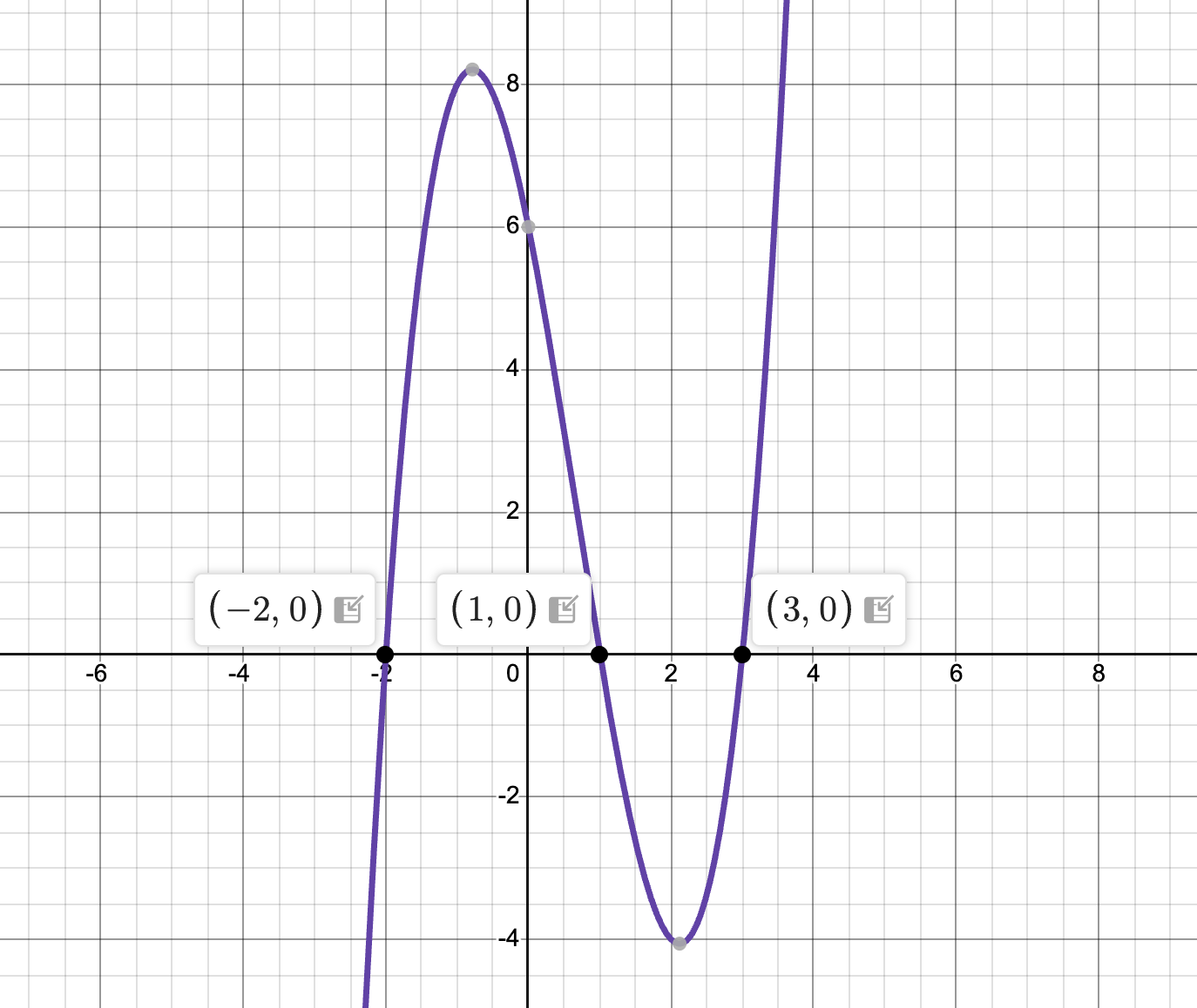
Here is what the graph looks like:

Graph of y=(x-1)(x+2)(x-3)

Made using Desmos

Looking Further

We will use very similar steps when solving polynomial inequalities, which some minor changes in the process.

Type a concept, like “slope” or “photosynthesis”.

↑ ↓ to choose · Enter to openSearch explanations and problems