পরিমিত ব্যবধান কাকে বলে?

Before this, knowগড়

Illustrated · 2 min

Standard Deviation

We've covered the measures of central tendency: mean, median, mode, and range.

Say you have two sets of numbers:

{−100,−50,−49,0,1,2,1000}\{-100, -50, -49, 0, 1, 2, 1000\} {−5,−4,−3,−2,−1,0,1,2,3,4,5}\{-5, -4, -3, -2, -1, 0, 1, 2, 3, 4, 5\}

There's something big to notice about the first set as opposed to the second set! Well, the numbers in the first set seem a lot more spread apart, while the numbers in the second set are closer together. Let's take a look at the means of the two sets.

The mean of the first set is around 115115 and the mean of the second set is 00. The mean for the second set makes sense - all the numbers are evenly spaced and fairly close to 00. For the first set, however, none of the numbers in the set seem to be close to the mean at all! That's because the numbers in the first set are very spread out.

There's actually a way to measure how 'spread out' numbers are: it's called the standard deviation (also represented by σ\sigma) of a data set.

Let's say that the government is looking at two schools: North School and South School. The South School has a much higher mean test score than the North School. The government's first reaction is to say that the kids at South School are smarter. But then they look at the standard deviation and see that it is quite large. This means that there are a few scores that aren't close to the mean, which increases the standard deviation.

The kids getting the high scores are only a very small part of the population of the school as a whole, so that doesn't necessary speak for the intelligence of the entire class. The government would have to look closer at the scores.

Graphically, here's what the standard deviation looks like on a normal set of data:

Standard deviation graph

Image source: By Caroline Kulczycky

The pink area represents the scores within one standard deviation away from the mean. These are the kids who score average or close to average. The turquoise area represents the kids who are one to two standard deviations from the mean. The kids in the left turquoise area maybe need to think about improving their scores while the kids on the right turquoise area are doing pretty well. The yellow area represents the kids who are two to three standard deviations away from the mean. On the left yellow area...well, those kids probably failed. But the right yellow area represents the kids who scored from 95%95\% to about a 100%100\%! They're doing really well!

Understanding the concept is very important, but here is the formula in case you actually want to calculate it!

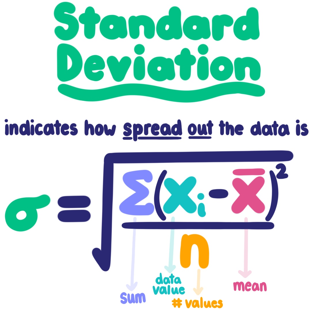
Standard deviation indicates how spread out the data is. σ=√[Σ(x-x̄)²/n]

Image source: By Caroline Kulczycky

In other words, σ=∑i=0n(xi−xˉ)2n\sigma = \sqrt{\frac{\sum_{i=0}^{n}(x_i-\bar{x})^2}{n}} xi= one of the data pointsxˉ= the meann= the total number of data points\begin{align} x_i &= \text{ one of the data points}\\ \bar{x}&=\text{ the mean}\\ n&= \text{ the total number of data points} \end{align} ∑i=0n(xi−xˉ)2\sum_{i=0}^{n}(x_i-\bar{x})^2 means that for each data point xi,x_i, find (xi−xˉ)2,(x_i-\bar{x})^2, then add all of those new values together (i.e., sum of squared values).

Interactive · 3 questions

Standard Deviation - What is it and how do I find it?

In these set of lessons, we're learning about the measures of central tendency. We'll learn about median, mode, mean, range, standard deviation, and statistical significance.

Standard deviation is a measure of how spread apart the numbers in a data set are. It is a single number that can help us figure out whether the numbers in the data set are clustered super close together or if there is a pretty wide range of values.

High standard deviation is represented by a wider bell curve, and low standard deviation is represented by a thinner bell curve.

Image source: By Caroline Kulczycky

Imagine that you make a histogram of your data. If you need a refresher on histograms, click here. Once you make a histogram, you can imagine a smooth curve tracing the tops of your bars, like the graphs above.

If you've got values that are all pretty close together (i.e., there's not much spread to the data), your curve will look like the one on the bottom. You can see that the curve is scrunched up (the technical term) - there is a low standard deviation. This tells us, just by looking at the graph, that there's not much variety or spread in our data.

If you've got values that are more spread out (i.e., there's more spread to the data), your curve will look like the one on the top. You can see that the curve is wider than the one on the bottom - there is a greater standard deviation.

Example

Data Set A: 2,11,15,19,43\text{Data Set A: } 2, 11, 15, 19, 43 Data Set B: 18,19,19,20,21\text{Data Set B: } 18, 19, 19, 20, 21

Of the two data sets above, which one has the largest standard deviation (σ\sigma)?

Choose one answer

Video · + 1 min read

(Video) Standard Deviation

by Math Meeting

Math Meeting has a good video on how to find the standard deviation and what it is.

Summary

Standard deviation measures how far apart or how close together the values in a data set are.

The formulas to calculate sample standard deviation and population standard deviation are slightly different. You use the first formula when your data points represent a smaller sample (a smaller sample size) of a bigger set of data. You use the second formula when you are dealing with a data set representing an entire population. In the formulas below, xˉ\bar{x} represents the mean, xix_i represents an arbitrary member of our data set, and the ∑\sum (i.e., the greek letter sigma) means you have to sum up the following values.

sample standard deviation=∑(xi−xˉ)2n−1\text{sample standard deviation} = \sqrt{\frac{\sum (x_i-\bar{x})^2}{n-1}} population standard deviation=∑(xi−xˉ)2n\text{population standard deviation} = \sqrt{\frac{\sum (x_i-\bar{x})^2}{n}}

Example

Let's look at what he does, step-by-step.

In the video, he finds the standard deviation of the following set of values: {1,2,3,4,5}\{1, 2, 3, 4, 5\}

First he finds the mean, xˉ:\bar{x}:

xˉ=1+2+3+4+55=155=3\bar{x} = \frac{1+2+3+4+5}{5} = \frac{15}{5} = 3

Then, for each xi,x_i, that is for each of the data points, he finds (xi−xˉ)2.(x_i-\bar{x})^2.

When xi=1,x_i=1, he calculates that (xi−xˉ)2=(1−3)2=(−2)2=4(x_i-\bar{x})^2 = (1-3)^2 = (-2)^2 = 4

When xi=2,x_i=2, he calculates that (xi−xˉ)2=(2−3)2=(−1)2=1(x_i-\bar{x})^2 = (2-3)^2 = (-1)^2 = 1

When xi=3,x_i=3, he calculates that (xi−xˉ)2=(3−3)2=(0)2=0(x_i-\bar{x})^2 = (3-3)^2 = (0)^2 = 0

When xi=4,x_i=4, he calculates that (xi−xˉ)2=(4−3)2=(1)2=1(x_i-\bar{x})^2 = (4-3)^2 = (1)^2 = 1

When xi=5,x_i=5, he calculates that (xi−xˉ)2=(5−3)2=(2)2=4(x_i-\bar{x})^2 = (5-3)^2 = (2)^2 = 4

Next, he finds ∑(xi−xˉ)2,\sum (x_i-\bar{x})^2, which is a fancy way of saying he adds up all the values we got for (xi−xˉ)2.(x_i-\bar{x})^2.

∑(xi−xˉ)2=4+1+0+1+4=10\sum (x_i-\bar{x})^2 = 4+1+0+1+4 = 10

Finally, he plugs everything into the appropriate formulas! First, he use the sample formula, and then the population formula. We know that n=5n=5 since there are 55 values in our dataset. So, plugging everything in, we get:

sample standard deviation=∑(xi−xˉ)2n−1=105−1≈1.58\text{sample standard deviation} = \sqrt{\frac{\sum (x_i-\bar{x})^2}{n-1}} = \sqrt{\frac{10}{5-1}} \approx 1.58 population standard deviation=∑(xi−xˉ)2n=105=2≈1.41\text{population standard deviation} = \sqrt{\frac{\sum (x_i-\bar{x})^2}{n}} = \sqrt{\frac{10}{5}} = \sqrt{2} \approx 1.41

If we want to extend this concept, we can use sample variance and confidence interval. Find the square root of the variance, and you'll find the standard deviation.

Type a concept, like “slope” or “photosynthesis”.

↑ ↓ to choose · Enter to openSearch explanations and problems