Interactive · 13 questions

+2 contributors



So we've learned about histograms and frequency distribution tables. Now, it's time to learn about the shape of the data and what it represents.
The Center and Spread
The first two are simple: center and spread. The center is where the data can be divided in half. The spread is the range of the data from the smallest to highest.
In later lessons, the center will be referred to as the median. We're learn more about spread when we learn about variance and standard deviation.
For an example, let's look at the following histogram:

Made using Desmos
Finding the center isn't always going to be as easy as looking at the midpoint of the -axis. This is because the larger the frequency of a bin, the more "weight" you have to add to it.
A good tactic is to add up all the frequencies: And then divide that in half. Now, we add up the frequencies from left to right, stopping when we reach . This is referred to as taking the cumulative frequency. Whatever bin you're in is the center.
Starting at bin we have a cumulative frequency of . Moving to bin we have a cumulative frequency of . Then, moving to bin goes to . Since this is over , we know the center is at bin .
The spread is from (lowest point) to (highest point).
Clusters and Gaps
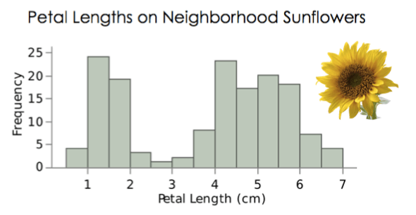
Next up, we have clusters and gaps. Clusters are subgroups the data could be broken into. Gaps are areas where there aren't any values.
Suppose we asked people ranging from years old to years old if they liked Pokemon. Then, we construct a histogram looking at the frequency of those who like Pokemon. We might see different clusters in the data set depending on if it was a kid, a teen, or an adult. If no one in an age range liked Pokemon, we would get a gap.
For a visual representation, let's look at the following histogram:

Made using Desmos
This graph has clusters. The first is from . The second is from . The third is from . The reason is two different clusters is because the data from has similar frequencies and the data from has similar frequencies.
From we have a gap. There is no data in this section.
Where is the center of this histogram?
What is the spread of this histogram?
Outliers and Modes
An outlier is a data point that is an extreme, and is usually found excluded from the rest of the data. An outlier can be the result of an error or it could be something that naturally came about.
Suppose you're using some machine to collecting data. While it's running, Jim, who sucks, knocks into the machine and disrupts it. Congratulations, you now have an outlier. All your data might be grouped together except for a single data point at a far end which was when Jim disrupted the machine.
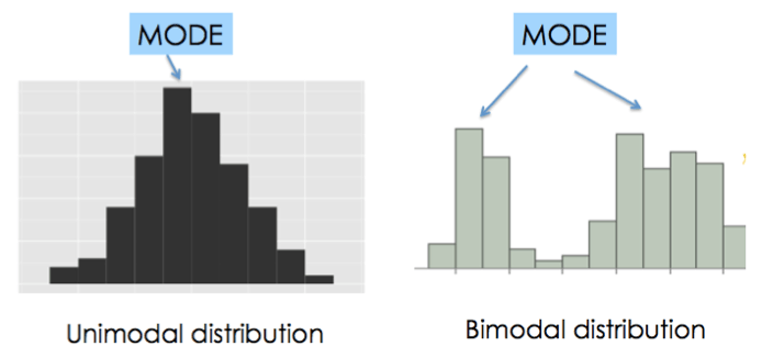
A mode is a major peak of a distribution. In other words, the interval with the highest frequency, or the interval that appears most often. There can be multiple modes in a distribution. If there's one mode we say it's unimodal. If there are two modes we say it's bimodal.
Let's look at the following histogram:
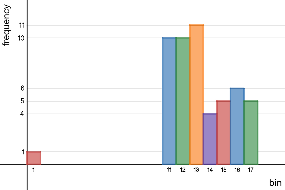
Made using Desmos
First up, we can see this histogram has an outlier at bin . This data point is isolated from the rest and has a small frequency.
Next, we look at modes. You might be tempted to say there is one mode (unimodal), but there are actually two (bimodal). The first mode is at bin since it is the highest. The second mode is at bin . This is because this bin is in it's own cluster and it's the highest for that cluster.
What is the center of this histogram?
What is the spread of the histogram?
How many clusters are there in the histogram?
Where is the gap in the histogram?
This type of data can also be represented in a bar graph or a pie graph, depending on the type of data you have. For example, if you have qualitative data that is based off of percents, then you may want to use a pie graph, because that type of graph shows parts of a whole or total number.
If you're just trying to represent a number of observations, a bar graph or histogram would be a good fit.
When deciding on types of graphs, it's not that they're mutually exclusive. You could have the same data that could be represented in different formats of graphs.
Shape
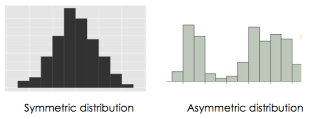
Finally, we have the shape of this distribution to look at. The first we look at is the symmetry. If the two halves of the distribution are mirror images, we say it's symmetric. If not, it's asymmetric.
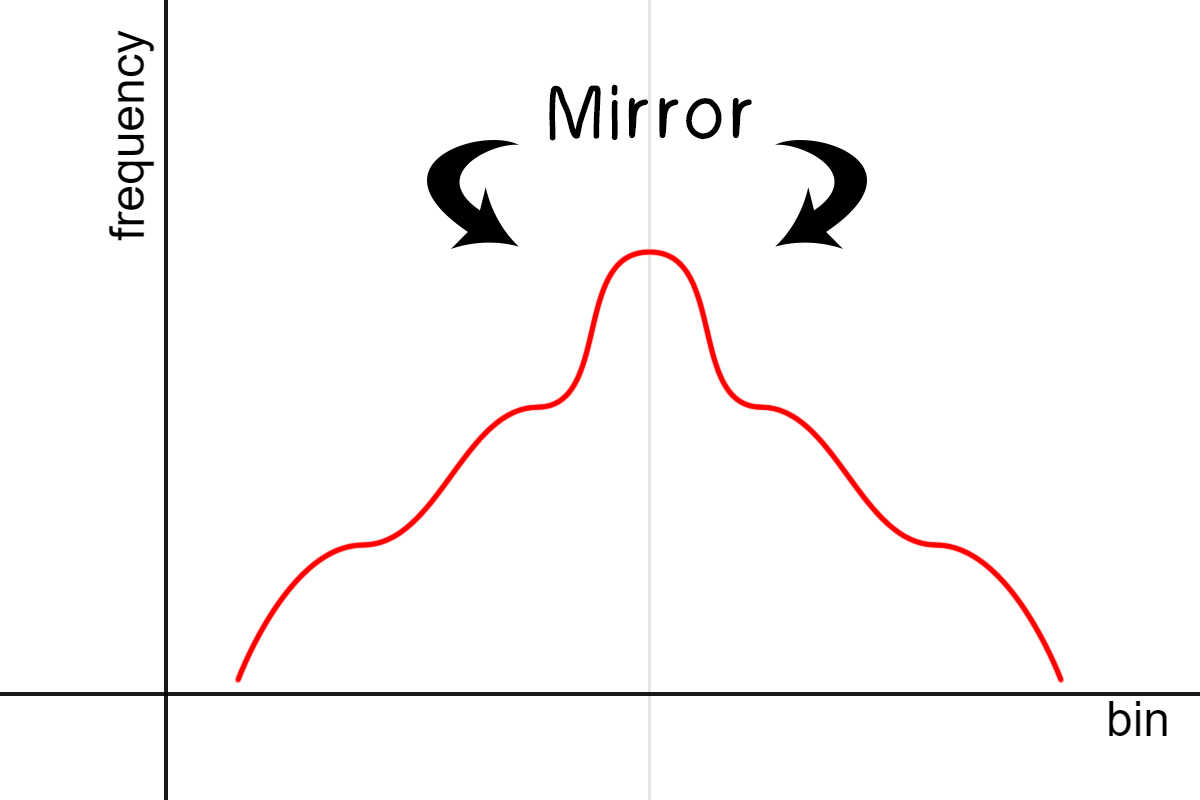
A symmetric graph.
Made using Desmos
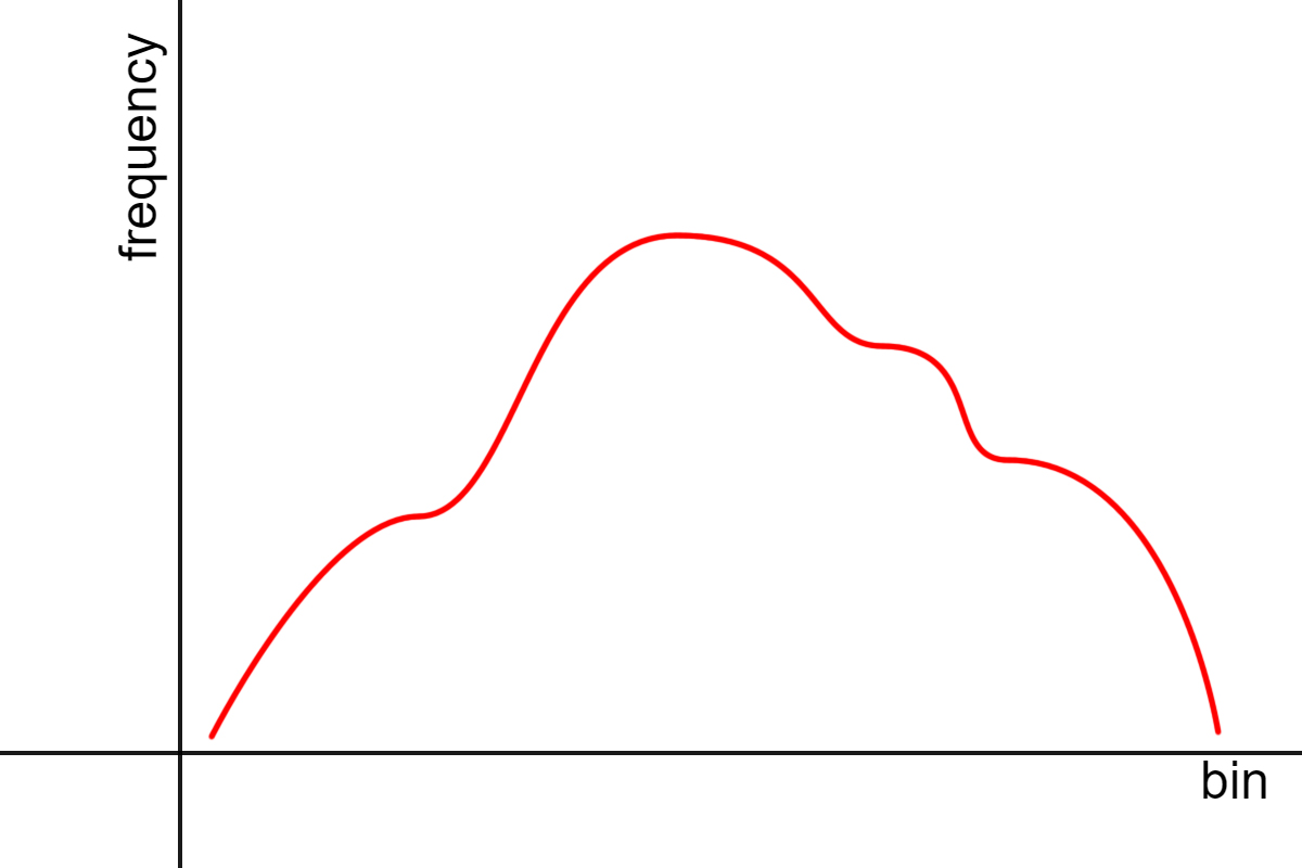
An asymmetric graph.
Made using Desmos
Next we have the skew. A distribution can be normal, skewed to the left, or skewed to the right.
A normal distribution has bell-shaped curve. It represents a group of similar data. An example would be the heights of people. Most of the population would be around a similar middle height. As you move to smaller heights or taller heights, it drops off and becomes less frequent.
A distribution that is skewed to the left, (also known as a negative skew) has a tail going towards the left of the graph (towards the negative numbers), with a hump on the right. A histogram of people diagnosed with dementia based on age would have a negative skew since there would be less cases in younger people and more cases in older people.
A distribution that is skewed to the right, (also known as a positive skew) has a tail going towards the right of the graph (towards the positive numbers), with a hump on the left. A histogram of people watching Saturday morning cartoons based on age would have a positive skew since there would be more kids watched and less adults.
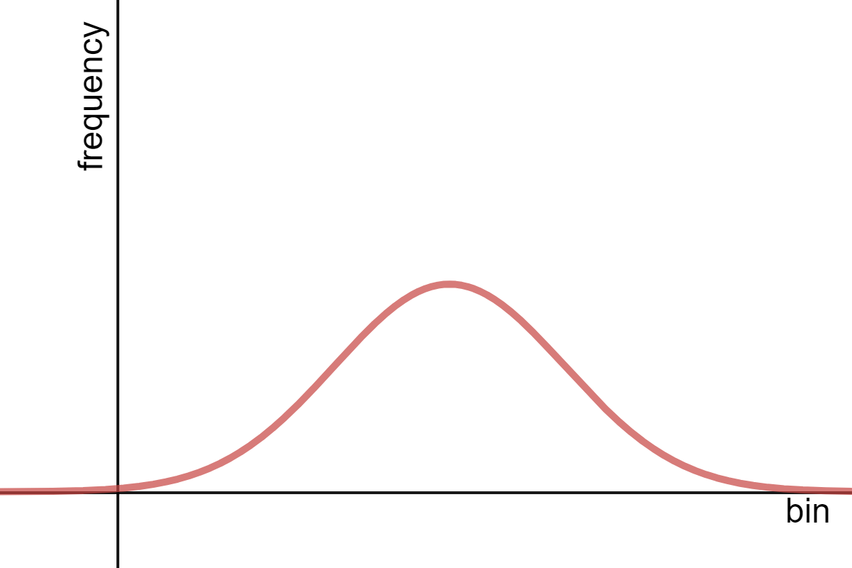
A normal distribution.
Made using Desmos
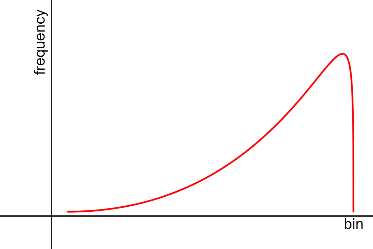
A skew to the left or a negative skew.
Made using Desmos
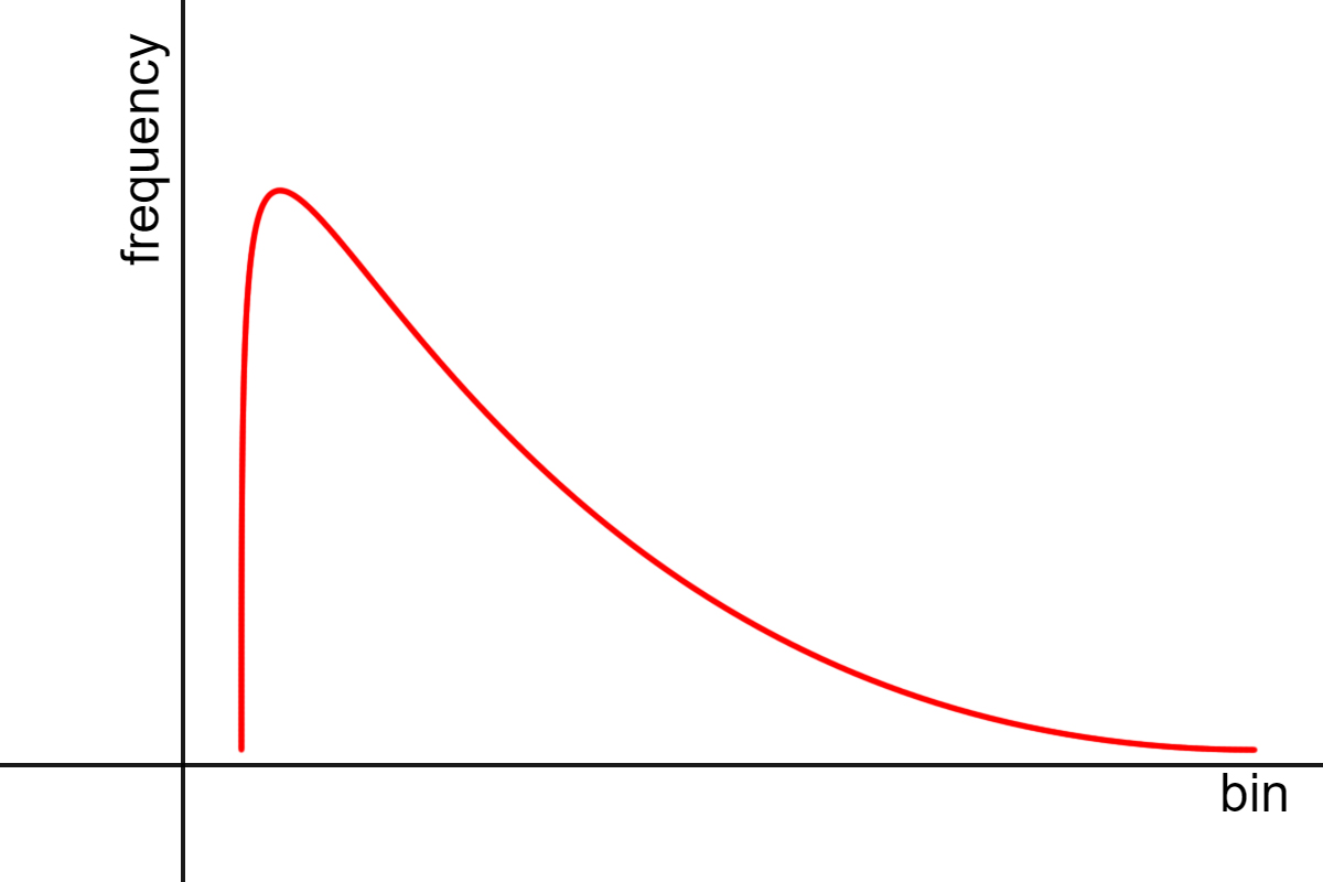
A skew to the right or a positive skew.
Made using Desmos
The final shape to look at is a uniform distribution. A uniform distribution is where all the data points are the same. It creates a horizontal line.
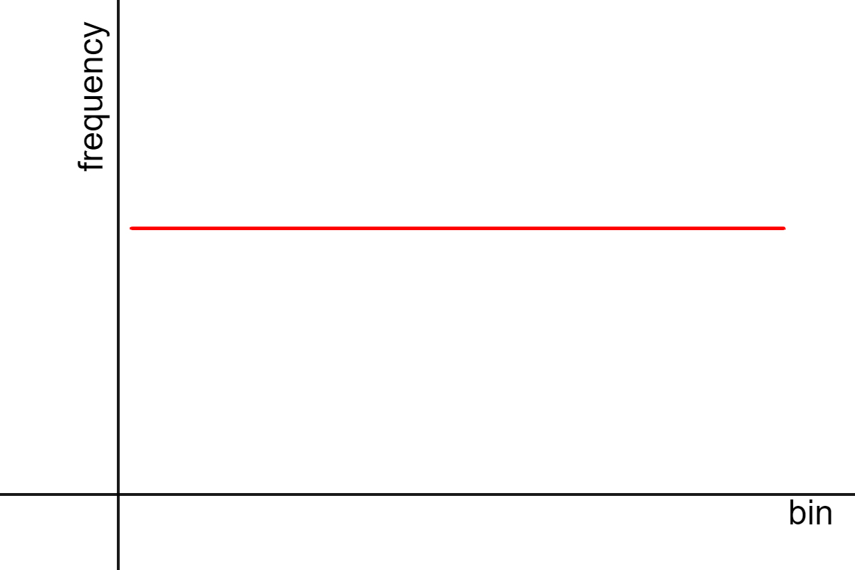
A uniform distribution.
Made using Desmos
So that was a lot of information, but it's finally over. Now, let's try some practice problems.
You can't stop watching Shrek 2! You decide to record your age every time you watch it. Turning it into a frequency table, you get:
First, turn this into a histogram:
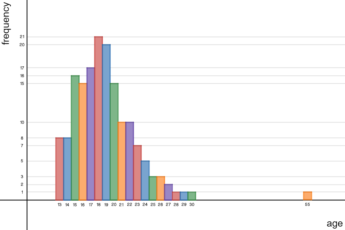
Made using Desmos
Select everything that describes this histogram.
Where is the center of the histogram?
What is the spread of the histogram?
Select the gap(s) in this histogram.
Select the outlier(s).
How many clusters are there?
What does the mode tell us in this histogram?