Here's a great video by PatrickJMT that shows you how to set up a matrix from a system of equations. He then shows you the 3 operations you use to solve the matrix.
To solve a system of equation using a matrix there are two basic steps.
1. Get all the pieces of the equations in the same order, with all the variables on one side and all the non-variable terms on the other.
2. Solve the matrix such that you have a diagonal of 1's on the left side of the matrix and a series of numbers (any numbers) in the rightmost column.
It's Step 2 that's complicated. Watch the first example in the video to find out how exactly to work through it, then pause and try the following problem. Note that since this one has three variables, it might be a bit trickier--if you have trouble, the video works through the same system of equations starting at 5:35.
x+2y+z=62x−y−z=1x+3y−4z=−3
Test Yourself: What is the solution to the system of equations above?
The answer is:
x=2y=1z=2
You can check your answer using the elimination or substitution methods, or by plugging the numbers into your original system of equations.
It might be helpful to review the elementary row operations in the previous lessons.
Setting Up the Matrix
We've been working with matrices for a while, so we know that we can manipulate matrices like we can manipulate equations and inequalities, but there are certain rules that only apply to matrices. We will use these techniques, specifically matrix row operations, to solve a system of equations.
To set this up we can use matrices to represent systems, so it's important to review that before applying row operations. As a review, we would represent the following system of equations,
{ax+by+czey+fz=d=g
with the following matrices:
[abecf]xyz=[dg]
The first matrix is called the coefficient matrix, the second matrix is called the variable matrix, and the third matrix is called the constant matrix (the column vector). If we think about the terms represented in the matrices, this nomenclature makes sense!
We can also represent this system using the following augmented matrix:
[abecfdg]
Matrix Row Operations
Now that we've set up our matrices, our next step is to use elementary matrix row operations to manipulate and solve the system. Matrix row operations include:
Row switching, where we can switch two rows in the matrix.
Row multiplication, where we can multiply all elements in a row by a constant value.
Row addition, where we can add the terms in one row to another row, and these values become the new values in the other row.
Let's think about why matrix row operations work when solving systems of equations. Because we are essentially doing the same thing as we would be doing if we were not using matrices. For example, remember with elimination, we would multiply all of the terms in one equation in order to make it easier to eliminate terms. That's similar to what we're doing with matrix row multiplication!
Our goal with using matrix row operations is to create row echelon form of a matrix, which is an augmented matrix in the following form:
100010001abc
a, b, and c will represent the solutions to our system of equations.
Do you notice the identity matrix in this augmented matrix? You'll learn more about matrices in row echelon form in linear algebra, but this is the basic concept that you can use to solve systems of equations.
Let's review: We will use matrix row operations to go from our original augmented matrix to this new matrix in row echelon form! However, sometimes it may be hard to get exactly this matrix in row echelon form, so we may simplify as much as possible before setting terms equal to each other to solve normally.
Let's walk through an example.
Example
Solve the following system of equations using matrix row operations.
⎩⎨⎧x+y+z2x+4y+2zx+2y+4z=2=4=2
Our first step is to make this into an augmented matrix:
121142124242
Now, we'll use our row operations to find the solution to this system of equations. Row operations will take a few steps, and there are multiple ways to reach the same solution! Be mindful of the row of a matrix you are working with.
R2=R2−2R1
101122104202
R3=R3−R1
100121103200
R2=2R2
100111103200
R1=R1−R2
100011103200
R3=R3−R2
100010103200
R3=3R3
100010101200
R1=R1−R3
100010001200
This is our final matrix in row echelon form! So, the solution to our system is x=2, y=0, and z=0.
Looking Further
Another method we did not talk about is gaussian elimination. This method is a little more complex, and you may commonly see it called row reduction.
There is one extra step we do to solve systems using matrix row operations.
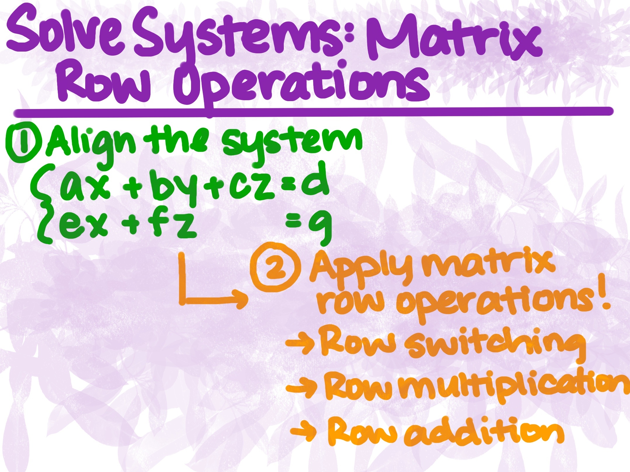
Image source: by Anusha Rahman
We've already learned the matrix row operations, including row switching, row multiplication, and row addition. We need to do one step before that to set up our system in matrix form.
We need to build an augmented matrix! Align the variables in the system, and that sets up your matrix.