Кусково лінійні функції

Before this, knowГрафіки функцій модуляГрафіки кусково заданих функцій

Illustrated · 2 min

Curve Approximations

We often learn about slope by studying linear functions. Early in algebra, you learn how to graph lines using slope-intercept form and point-slope form.

But linear functions are not the only ones that have slope. In fact, all functions have slope.

Linear functions have a constant slope, which means the slope stays the same everywhere. Nonlinear functions are different. Their slope can change from point to point on the graph.

In higher-level math, you use a derivative to find the slope at any point on a curve. For now, we can use linear approximation to estimate the slope of a curve near a point.

Let's take a look at the graph of the function y=x2y=x^2 when x≥0x\ge0. The domain is the set of real numbers greater than zero.

Only the right side of the parabola y=x^2. It's a smooth curve that goes up and to the right

Made with Demos

This function is made up of a smooth curve.

To study it, we will create a linear piecewise function by connecting points along the graph. This will help us find the average slope between each pair of points.

We’ll start by placing a point every 2.52.5 units along the xx-axis.

Now we have points at (0,0), (2.5,6.25), and (5, 25)

Made with Desmos

Now we can connect these points. We have the points (0,0)(0,0), (2.5,6.25)(2.5,6.25), and (5,25)(5,25). Let's find the slopes between the points. m1=y2−y1x2−x1m1=6.25−02.5−0m1=6.252.5m1=2.5m2=y3−y2x3−x2m2=25−6.255−2.5m2=18.752.5m2=7.5\begin{align}m_1&=\frac{y_2-y_1}{x_2-x_1}\\ m_1&=\frac{6.25-0}{2.5-0}\\ m_1&=\frac{6.25}{2.5}\\ m_1&=2.5\\ \\ m_2&=\frac{y_3-y_2}{x_3-x_2}\\ m_2&=\frac{25-6.25}{5-2.5}\\ m_2&=\frac{18.75}{2.5}\\ m_2&=7.5 \end{align} We can use the slopes to find the equations of each line in our piecewise model. y−y1=m(x−x1)y−0=2.5(x−0)y=2.5x\begin{align}y-y_1&=m(x-x_1)\\ y-0&=2.5(x-0)\\ y&=2.5x \end{align} This will be the equation for the line between x=0x=0 and x=2.5x=2.5. y−y2=m(x−x2)y−6.25=7.5(x−2.5)y−6.25=7.5x−18.75y=7.5x−12.5\begin{align}y-y_2&=m(x-x_2)\\ y-6.25&=7.5(x-2.5)\\ y-6.25&=7.5x-18.75\\ y&=7.5x-12.5 \end{align} This will be the equation for the line between x−2.5x-2.5 and x=5x=5. The entire piecewise function will be: y={2.5x0≤x<2.57.5x−12.52.5≤x≤5y=\begin{cases}2.5x &0\le x<2.5\\ 7.5x-12.5 &2.5 \le x \le 5 \end{cases} Let's take a look at this on the graph.

Now we have lines to connect the points. We can see the average slope at different points on the graph

Made with Desmos

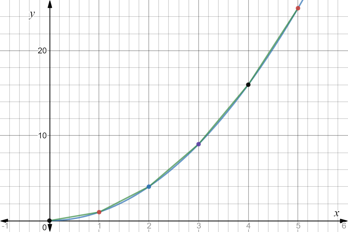
The slope of the first line, 2.52.5, is the average slope of the function over 0≤x<2.50 \le x <2.5. The slope of the second line, 7.57.5, is the average slope of the function over 2.5≤x≤52.5 \le x \le 5. We can make these estimations more accurate to the true values of the curve by making the gaps in between the points. Here is this same process done for a point every 11 unit on the xx-axis.

The points are closer together and the lines have a better fit to the curve. This is true every time you increase the number of steps in the piecewise function.

Made with Desmos

The more frequent steps give us a better fitting piecewise function. Let's zoom in one more time with a point every 0.50.5 units on the xx-axis.

The piecewise approximation is an even tighter fit to the parabola.

Made with Desmos

This gives us an even closer fit to the curve.

We could keep breaking the curve into smaller and smaller pieces. Eventually, the pieces would be so small that they would look almost the same as the original curve.

At that point, the linear pieces closely match the shape of the curve.

Useful Equations

You need to remember that you are just working with linear equations you are used to.

Slope: m=y2−y1x2−x1m=\frac{y_2-y_1}{x_2-x_1}

Point-Slope Form: y−y1=m(x−x1)y-y_1=m(x-x_1)

Wrap-Up

We can use small line segments in a piecewise function to estimate the average slope of a curve.

The smaller the line segments are, the more accurate the estimate becomes. This is because the lines match the curve more closely.

This idea leads into calculus, where we learn about derivatives. Derivatives help us find the exact slope of a curve at a single point.

Video

(Video) PIecewise Linear Functions

by Kirk Weiler

Here's a video by Kirk Weiler going over piecewise linear functions. He works through some common problems involving the topic.

Summary

A piecewise linear function is a function whose rule consists of multiple linear equations.

To start with, best practice is to fully graph both roles in the function. However - that may violate the fundamental rule of a function, where there is just one yy value for every xx value.

That's why piecewise functions have intervals, which tell you over what intervals, or values of xx, the function is true for. So, you'll graph the function as usual, but you will only keep the parts that are within the internal.

Illustrated · 1 min

Piecewise Linear Functions

A linear piecewise function is a function made up of different lines.

Each line works over a specific interval of input values. This means one rule applies for part of the graph, and a different rule applies for another part.

Together, these lines form one complete function.

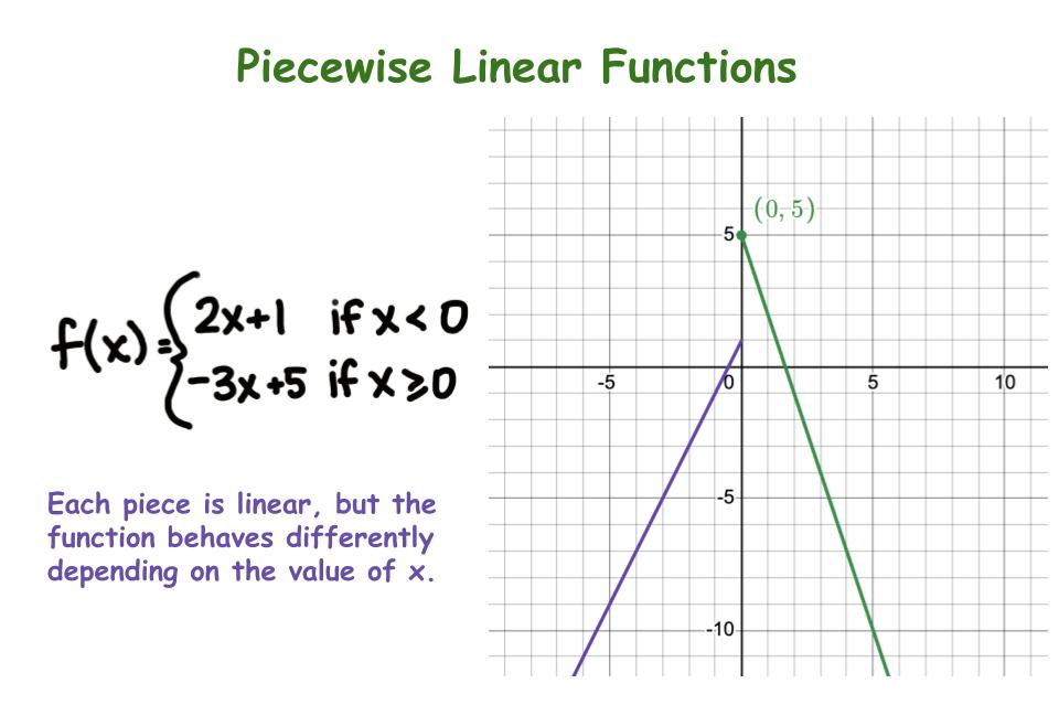
Piecewise Linear Functions: Each piece is linear, but the function behaves differently depending on the value of x.

Made using Desmos

Basically, the function has different rules for different ranges of xx values. Each rule is a straight line (which is why we call it linear!).

In the above function,

  • When xx is less than 00, the function follows the line 2x+12x+1
  • When xx is 00 or greater, the function follows the line −3x+5-3x+5

####What Makes It Different

A piecewise function is a function that follows different rules for different parts of its graph.

Some piecewise functions use straight lines, but not all of them do. Others can use curves or different types of equations.

We have talked about piecewise functions before, so this idea should feel familiar.

Type a concept, like “slope” or “photosynthesis”.

↑ ↓ to choose · Enter to openSearch explanations and problems