微分中值定理

Steven Kwon has written about the intuition and proof behind the MVT here.

But why do we need the Mean Value Theorem (MVT)?

Well, the MVT tells us that for any interval $[a,b]$, we can find an interior point $c\in (a,b)$ where the derivative/"sensitivity" $f'(c)$ "represents" the overall change of the function, in the sense that $\Delta{f} = f(b)-f(a)$ equals $f'(c)\Delta{x} = f'(c)(b-a)$.

So the rough answer is that if we have information about the derivative/"sensitivity" of a function at lots of points (e.g. on an interval $[a,b]$), then we can use the MVT to translate that into properties of the function itself. For example, in (1) below, we're given lots of "local" derivative information, e.g. that $f'(x) > 0$ always (the derivative is always positive), and we can use MVT to translate that into a more "global" statement about increasing functions (i.e. $f(a) < f(b)$ whenever $a < b$).

Well, the rough answer is that it allows us to use "local" derivative/"sensitivity" information to say interesting things about "global"/big-picture function properties. (The limit definition of a derivative already tells us how to use "global"/big-picture function information---namely the function values themselves---to say interesting things about "local" derivative/"sensitivity" properties.) In applications 1, 2, and 3 below, this is how the MVT is used. *

On the other hand, the MVT can seem kind of arbitrary (&), especially if you don't care so much about rigor. Is it really necessary to learn/teach?

Well, you can read the thread if you're interested. But for me, here's the key takeaway, stolen from Jeff Strom's excellent answer:

The MVT is the basis for all proofs that geometric intuition about slopes of tangent lines holds for the limit definition. That is, the metamathematical content of the MVT is that the intuition definition matches the formal definition.

In other words, the MVT is just a rigorous way to capture our geometric intuition about derivatives, which you use a lot in sketching derivatives. But again, don't worry if you find the MVT arbitrary. You'll be fine if you understand the intuition for some of its most important applications:

(1) Increasing and decreasing (monotone) functions in terms of derivatives.

(2) Functions with always-zero derivatives (this is later applied to answer the very important question of whether anti-derivatives are unique, but don't worry if you haven't heard of anti-derivatives yet).

(3) When tangents lie above or below graphs.

In all of these, we have some intuition involving some sort of inequality (&&) in a function or graph: the notion of increasing/decreasing in (1), a graph "resembling a horizontal line everywhere" in (2), and the notion of above/below in (3). And in each case, the MVT is just a simple way to formalize our graphical intuition.

(4) Precursor to Taylor's "Weak" Theorem *

Additional comments (feel free to ignore these)

(&) The reason MVT seems arbitrary is because it just says there exists some point $c$ with $f'(c) = \frac{f(b)-f(a)}{b-a}$, while it would possibly be more natural to have a statement like "the average value of the derivative is $\frac{f(b)-f(a)}{b-a}$". And it turns out that this is true, in some sense (it's half of the fundamental theorem of calculus, which you'll encounter later on). The caveat? To prove that, we use (2) from above, which comes from MVT.

(&&) More precisely, it's worth clarifying why MVT works to prove these inequalities, because (&) makes MVT seem kind of unnatural or artificial. Roughly speaking, the reason MVT works for 1, 2, and 3 is that the information on derivatives we have in these cases is uniform:

(1) We're using MVT on a function with $f'(x) > 0$ for all $x$.

(2) We're using MVT on a function with $f'(x) = 0$ for all $x$.

(3) We're using MVT on a function with $f''(x) > 0$ for all $x$.

In the previous section, we talked about Rolle's theorem, which stated that given a function $f(x)$ continuous on $[a,b)$ and differentiable on $(a,b)$, if $f(a)=f(b)$ there exists a $c$ in $(a,b)$ such that $f'(c)=0$. Now, what if $f(a)\ne f(b)$? Can a similar case hold?

Thankfully, the answer is yes, and this leads us to the Mean Value Theorem for derivatives. (We specify that this is for derivatives, because there is also a Mean Value Theorem for integrals, which you will see later.)

Before we tell you the theorem, let's see if we can figure it out together: consider the function $f(x)=x^2$ on the interval $[0,1]$, as shown below:

As we suggested, let's try rotating the graph so that $b$ lies on the $x$-axis:

Aha! if we call this rotated function $g(x)$, we have $g(a')=g(b')=0$. So, by Rolle's Theorem we know there exists a $c'$ in $(a',b')$ such that $g'(c')=0$.

From here, if we rotate the graph back to its original position, we'll get the following picture:

Aha! So it seems like in the interval $(a,b)$, there's a point for which the tangent line going through it is parallel to the line through the endpoints! That's exactly what the Mean Value Theorem states. Formally, it says the following:

Mean Value Theorem (for derivatives): Suppose $f(x)$ is a function continuous on $[a,b]$ and differentiable on $(a,b)$. Then there exists a $c$ with $a<c<b$ such that $$f'(c)=\frac{f(b)-f(a)}{b-a}.$$

Notice that the right hand side is simply the expression for the slope of the line going through the endpoints $(a,f(a))$ and $(b,f(b))$, so this is exactly what we just discovered graphically.

We also observe that when $f(a)=f(b)$, the right hand side becomes $0$, in which case we get back Rolle's Theorem. So, we can see that Rolle's Theorem is just a special case of the Mean Value Theorem.

Okay! Now that we know the theorem, let's look at an example: suppose we have $f(x)=x^2$ on the interval $[0,2]$, as shown below:

Let's try to find a value of $c$ that satisfies the Mean Value Theorem. To do so, we plug in the appropriate values into the equation given above: $$f'(c)=\frac{f(b)-f(a)}{b-a}=\frac{f(2)-f(0)}{2-0}=\frac{f(2)-f(0)}{2}.$$ Since $f(x)=x^2$, we have $f'(x)=2x$, and so the equation becomes $$f'(c)=2c=\frac{f(2)-f(0)}{2}=\frac{2^2-0^2}{2}=2.$$ Solving for $c$ yields $c=1$. Since this is in the interval $(0,2)$, we have found our value of $c$ that satisfies the Mean Value Theorem.

Now you try!

First, let's graph the function, to get a better picture:

As before, we plug in the appropriate values in the given equation: $$f'(c)=\frac{f(b)-f(a)}{b-a}=\frac{f(2)-f(-1)}{2-(-1)}=\frac{f(2)-f(-1)}{3}.$$ Since $f(x)=x^3-2x$, we have $f'(x)=3x^2-2$. So, we get $$f'(c)=3c^2-2=\frac{f(2)-f(-1)}{3}=\frac{[2^3-2(2)]-[(-1)^3-2(-1)]}{3}=1.$$ Solving for $c$, we get $$3c^2=3\Longrightarrow c=\pm 1.$$ We get two values of $c$, but only $c=1$ is strictly between $-1$ and $2$. So, that's our value of $c$ that satisfies the Mean Value Theorem. [But don't be discouraged: in general we can have more than one value of $c$ that works.]

Again, we now know how to use the Mean Value Theorem in calculations. But can we also use this to prove other results in calculus?

Of course, the answer is yes. In fact, the Mean Value Theorem is one of the most important theorems in calculus, because it can be used to prove many theorems like L'Hospital's Rule. For now, try and use the Mean Value Theorem to prove the following proposition:

Proposition: Suppose $f(x)$ is continuous on $[a,b]$ and differentiable on $(a,b)$. If $f'(x)=0$ for all $x$ in $(a,b)$, then prove that $f(x)$ is constant.

Choose a point $p$ in the interval $(a,b)$. By the Mean Value Theorem, there exists $r$ in $(a,p)\subset (a,b)$ such that $$f'(r)=\frac{f(p)-f(a)}{p-a}.$$ Since $(a,p)$ is a subset of $(a,b)$, it is given that $f'(r)=0$, which means that $$0=\frac{f(p)-f(a)}{p-a}\Longrightarrow f(p)-f(a)=0\Longrightarrow f(p)=f(a).$$ So, for any $p$ in the interval $(a,b)$, we just showed that $f(p)=f(a)$. Thus, we can conclude that $f(x)$ is constant over the entire interval.

Like in this example, the Mean Value Theorem becomes very important in the following sections as well. So, read on to find out more!

Now, we will use Rolle's Theorem to prove the Mean Value Theorem: Suppose $f(x)$ is continuous on $[a,b]$ and differentiable on $(a,b)$. Consider a new function $$g(x)=f(x)-(x-a)\frac{f(b)-f(a)}{b-a}.$$ Since this is just the sum of $f(x)$ and a linear function, it is also continuous and differentiable wherever $f(x)$ is. Also, we see that $$g(a)=f(a)-(a-a)\frac{f(b)-f(a)}{b-a}=f(a)-0=f(a),$$ while $$g(b)=f(b)-(b-a)\frac{f(b)-f(a)}{b-a}=f(b)-(f(b)-f(a))=f(a).$$ Thus, we have $g(a)=g(b)$, and so by Rolle's Theorem we know there exists $c$ with $a<c<b$ such that $g'(c)=0$. But $$g'(x)=\frac{d}{dx}\left(f(x)-(x-a)\frac{f(b)-f(a)}{b-a}\right)=f'(x)-\frac{f(b)-f(a)}{b-a}.$$ Thus, $$g'(c)=0=f'(c)-\frac{f(b)-f(a)}{b-a}.$$ This shows that $$f'(c)=\frac{f(b)-f(a)}{b-a},$$ as desired.

Here is a worksheet to practice your newly learned skill: applying the Generalized Rolle's Theorem (a.k.a Mean Value Theorem). Good luck! P.S. Answers are on the bottom.

(Video) The Mean Value Theorem

by PatrickJMT

Here's a video by patrickJMT explaining the Mean Value Theorem and how it is used.

The Mean Value Theorem states that some function, $f(x)$, is

1. Continuous on $[a,b]$
2. Differentiable on $(a,b)$

then there exists at least one point, $c$, in $(a,b)$ such that $$f'(c)=\frac{f(b)-f(a)}{b-a}$$

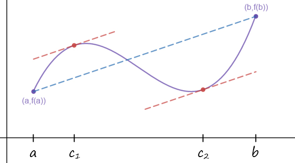
Graphic Representation

Suppose we have some function on the interval $(a,b)$ that's continuous and differentiable.

Now we take a line that connects point $a$ to point $b$.

This line is the slope between the two points and can be written as: $$m=\frac{f(b)-f(a)}{b-a}$$

We see that there are places on this graph where the slope of the derivative at that point is equal to this line through the middle.

The Mean Value Theorem tells us there will be at least one point whose derivative is equal to the slope of the endpoints. In this example we have two: $c_1$ and $c_2$. $$f'(c_1)=m\\ f'(c_2)=m$$

Let's try a problem involving the Mean Value Theorem.

For $f(x)=1+\sqrt[3]{x-1}$ on the interval $[2,9]$, find all $c$ in $[2,9]$ such that: $$f'(c)=\frac{f(9)-f(2)}{9-2}$$

We first need to show that the function is continuous and differentiable on this domain. There's actually a theorem that states root functions are continuous on their domains.

To find where a function is differentiable you just find the domain of its derivative. $$\begin{align} f(x)&=1+\sqrt[3]{x-1}\\ f'(x)&=\frac{1}{3}(x-1)^{-\frac23}\\ f'(x)&=\frac{1}{3(x-1)^{\frac23}} \end{align}$$ The derivative is undefined where the denominator equals zero. $$\begin{align} 3(x-1)^{\frac23}&=0\\ x-1&=0\\ x&=1 \end{align}$$ So the derivative is undefined at $x=1$. Since our interval doesn't contain this point we know our function is differentiable within the domain.

Since our function is continuous and differentiable on this domain, we can use the Mean Value Theorem. $$\begin{align} f'(c)&=\frac{f(9)-f(2)}{9-2}\\ \frac{1}{3(c-1)^{\frac23}}&=\frac{[1+\sqrt[3]{9-1}]-[1+\sqrt[3]{2-1}]}{7}\\ \frac{1}{3(c-1)^{\frac23}}&=\frac{3-2}{7}\\ \frac{1}{3(c-1)^{\frac23}}&=\frac{1}{7}\\ 3(c-1)^{\frac23}&=7\\ (c-1)^{\frac23}&=\frac73\\ c-1&=\bigg(\frac73\bigg)^{\frac32}\\ c&=1\pm\sqrt{\bigg(\frac73\bigg)^3} \end{align}$$

The only one that's within our interval is: $$c=1+\sqrt{\bigg(\frac73\bigg)^3}$$ This is the point where the derivative equals the slope of the endpoints.