曲线的图形分析词汇表

(Videos) Summary of Curve Sketching

by PatrickJMT

Here's a set of videos by patrickJMT where he shows you how to do a full blown analysis on a function in order to graph it. We're talking all the tests, tricks, and topics that have been covered up to and including calculus when it comes to graphing. All in one convenient place.

In these videos he goes over:

1. Domain
2. Intercepts
3. Symmetry
4. Asymptotes
5. Intervals of Increase/Decrease
6. Local Max/Mins
7. Concavity
8. Sketching the Graph

The luckily function we're looking at tonight is $$f(x)=\frac{x}{\sqrt{x^2+1}}$$ Let's begin.

Domain

The domain of a function is all the possible $x$ values of that function. When finding the domain of a function we basically just want to find any values where our function becomes undefined. Some examples would be a zero in the denominator or a square root sign with a negative value.

Luckily, for us our function can have both of these happen so we need to figure out where it happens and exclude those points from the domain.

First, let's find where our denominator equals zero. $$\begin{align} \sqrt{x^2+1}&=0\\ x^2+1&=0\\ x^2&=-1\\ x&=\sqrt{-1} \end{align}$$

Since we got an imaginary number, we can conclude that there's no value of $x$ that makes our function's denominator zero. So far so good. Let's now check to make sure we don't get any negative values inside our square root.

$$\begin{align} x^2+1&<0\\ x^2&<-1\\ x&<\sqrt{-1} \end{align}$$

Again, since we got an imaginary number, we can conclude that there's no value of $x$ that makes a negative value inside the square root.

So our domain is all real numbers, $\mathbb{R}$, or $(-\infty,\infty)$.

Intercepts

The intercepts are the points where the function crosses either the $y$-axis or the $x$-axis. To find these, we set either the $x$ values equal to zero or the $y$ values equal to zero.

Let's start with the $y$-intercept. To find this we set $x=0$. $$\begin{align} f(x)&=\frac{x}{\sqrt{x^2+1}}\\ f(0)&=\frac{\color{red}{(0)}}{\sqrt{\color{red}{(0)}^2+1}}\\ &=0 \end{align}$$

So our function crosses the $y$ axis at $0$. In other words, we know that the point $(0,0)$ is on the graph.

If you think about it, the point $(0,0)$ is also an $x$ intercept but we'll still work through it to show this.

Let's find the $x$ intercept now by letting $y$ ($f(x)$) equal zero. $$\begin{align} \frac{x}{\sqrt{x^2+1}}&=0\\ x&=0 \end{align}$$

This tells us we have an $x$ intercept at $(0,0)$.

Symmetry

A function is considered even if $f(-x)=f(x)$. This means if we plug in a negative value we get the answer we would if we plugged in its positive counterpart. If a function is even it is symmetric about the $y$-axis.

A function is considered odd if $f(-x)=-f(x)$. This means the function is symmetric about the origin; the line $y=x$.

So we test our function by plugging in $-x$. $$\begin{align} f(x)&=\frac{x}{\sqrt{x^2+1}}\\ f(-x)&=\frac{\color{red}{(-x)}}{\sqrt{\color{red}{(-x)}^2+1}}\\ &=-\frac{x}{\sqrt{x^2+1}} \end{align}$$

Notice how we got out the negative version of the function we started with. Therefore our function is odd and it is symmetric about the origin.

Asymptotes

A vertical asymptote is a point where the function is some nonzero value over zero. $$\frac{\text{nonzero}}{0}$$ But we already looked at this when we looked at domain. We set the denominator equal to zero and found there were no points where this happens. So, there's no vertical asymptotes in our graph.

To find a horizontal asymptote we need to look at $\lim\limits_{x\rightarrow-\infty}f(x)$ and $\lim\limits_{x\rightarrow\infty}f(x)$.

Let's look at when $x\rightarrow\infty$. $$\lim_{x\rightarrow\infty}\frac{x}{\sqrt{x^2+1}}=\frac{\infty}{\infty}$$

We need to apply a trick to be able to take this limit since it gives us infinity over infinity. For a closer look at how to do this, watch his previous video.

Look in the denominator and choose the largest power. In this case, it's $x^2$. But it's also under a square root so we need to apply this to the largest power we selected, $\sqrt{x^2}=x$. This result is what we divide the numerator and denominator by.

$$\begin{align}\frac{\frac{1}{x}x}{\frac1x\sqrt{x^2+1}}&=\frac{1}{\sqrt{\frac1{x^2}}\sqrt{x^2+1}}\\ &=\frac{1}{\sqrt{\frac{1}{x^2}(x^2+1)}}\\ &=\frac{1}{\sqrt{1+\frac1{x^2}}} \end{align}$$

Now if we take the limit we get a better answer. \begin{align}\lim_{x\rightarrow\infty}\frac{1}{\sqrt{1+\frac1{x^2}}}&=\frac{1}{\sqrt{1+\frac{1}{\infty}}}\ &=\frac{1}{\sqrt{1+0}}\ &=1 \end{align}

So we now know that $y=1$ is a horizontal asymptote.

Next, let's check the limit at negative infinity. $$\lim_{x\rightarrow-\infty}\frac{x}{\sqrt{x^2+1}}=\frac{-\infty}{\infty}$$

We still have to divide by the highest power in our denominator, like above. $$\frac{\frac1xx}{\frac1x\sqrt{x^2+1}}$$

But there's one caveat to be weary of. It's incorrect to just square this term and put it under a radical sign like so: $$\frac{\frac1xx}{\sqrt{\frac1{x^2}}\sqrt{x^2+1}}\color{red}{\text{ Incorrect.}}$$

If we plug a negative number into $\frac1x$ we get out a negative answer. But if we plug a negative number into $\sqrt{\frac1{x^2}}$ we get out a positive answer. So these two are not equal. To fix this we need to place a negative sign out front. $$\frac{\frac1xx}{\color{red}{-}\sqrt{\frac1{x^2}}\sqrt{x^2+1}}\color{green}{\text{ Correct.}}$$

So now let's take the limit. \begin{align}\lim_{x\rightarrow-\infty}\frac{1}{-\sqrt{1+\frac1{x^2}}}&=\frac{1}{-\sqrt{1+\frac{1}{-\infty}}}\ &=\frac{1}{-\sqrt{1+0}}\ &=-1 \end{align}

So we have a second horizontal asymptote at $y=-1$.

Increasing and Decreasing

To figure out where the graph is increasing or decreasing we need to look at the derivative. $$\begin{align} f(x)&=\frac{x}{\sqrt{x^2+1}}\\ f'(x)&=\frac{\color{red}{[x]'}\sqrt{x^2+1}-x\color{red}{[\sqrt{x^2+1}]'}}{[\sqrt{x^2+1}]^2}\\ &=\frac{\sqrt{x^2+1}-x\cdot\frac{1}{2\sqrt{x^2+1}}\cdot\color{red}{[x^2+1]'}}{x^2+1}\\ &=\frac{\sqrt{x^2+1}-x\cdot\frac{1}{2\sqrt{x^2+1}}\cdot2x}{x^2+1}\\ &=\frac{\sqrt{x^2+1}-\frac{2x^2}{2\sqrt{x^2+1}}}{x^2+1}\\ &=\frac{\sqrt{x^2+1}-\frac{x^2}{\sqrt{x^2+1}}}{x^2+1}\\ &=\frac{\frac{x^2+1}{\sqrt{x^2+1}}-\frac{x^2}{\sqrt{x^2+1}}}{x^2+1}\\ &=\frac{\frac{1}{\sqrt{x^2+1}}}{x^2+1}\\ &=\frac{1}{(x^2+1)^{\frac32}}\\ \end{align}$$

Once you have the derivative find the values of $x$ that make it zero or undefined. These will be your critical points.

If we try to set this derivative equal to zero and solve you'll find we get a false statement which means there's no solution. $$\begin{align} \frac{1}{(x^2+1)^{\frac32}}&=0\\ 1&=0 \end{align}$$

To make the derivative undefined we would want the denominator to equal zero. But again you'll find that there are no solutions. $$\begin{align} (x^2+1)^{\frac32}&=0\\ x^2+1&=0\\ x^2&=-1\\ \end{align}$$

So this function doesn't have any critical points. But we can still test if the function is increasing or decreasing. Just take any number within the interval $(-\infty,\infty)$ and plug it into the derivative. \begin{align} f'(0)&=\frac{1}{(\color{red}{(0)}^2+1)^{\frac32}}\ &=1 \end{align} Since the derivative comes out positive, we know the function is increasing on this interval, or always increasing. $$(-\infty,\infty)\ \nearrow$$

Local Extrema

Because our function is always increasing, we know there will be no local maximums and no local minimums.

Concavity

To look at concavity we need the second derivative of our function. \begin{align} f'(x)&=\frac{1}{(x^2+1)^{\frac32}}\ &=(x^2+1)^{-\frac32}\ f''(x)&=-\frac32(x^2+1)^{-\frac52}\cdot\color{red}{[x^2+1]'}\ &=\frac{-3}{2(x^2+1)^{\frac52}}\cdot2x\ &=\frac{-3x}{(x^2+1)^{\frac52}} \end{align}

Again, we need to find where our derivative equals zero or is undefined. Let's set it equal to zero first. $$\begin{align} \frac{-3x}{(x^2+1)^{\frac52}}&=0\\ -3x&=0\\ x&=0 \end{align}$$

We should also set the denominator equal to zero to see where it's undefined but this will yield no solution like above.

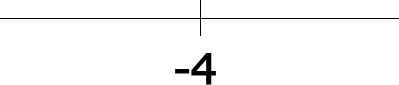
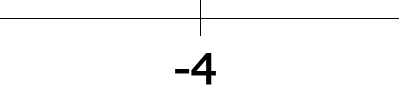
So our sign chart would look like

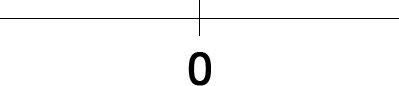
Choose a point within each of these intervals and plug it into the second derivative to find its sign.

If we plug in a negative number we get a positive over a positive which is a positive number. This means the graph is concave up on this interval. $$(-\infty,0)\ CU$$

If we plug in a positive number we get a negative over a positive which is a negative number. This means the graph is concave down on this interval. $$(0,\infty)\ CD$$

Because the graph switches concavity at $0$ we call it an inflection point.

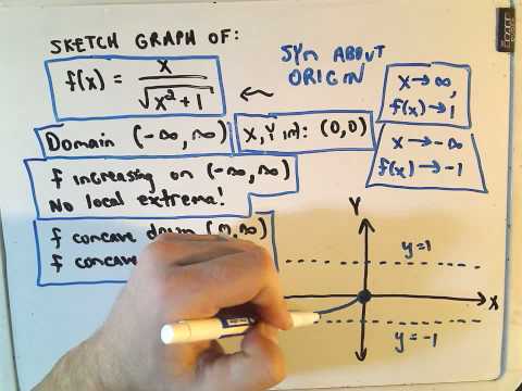
Recap

$$f(x)=\frac{x}{\sqrt{x^2+1}}$$

• Symmetric about the origin.
• Domain $(-\infty,\infty)$
• $x$ and $y$ intercept at $(0,0)$
• Horizontal asymptotes at $y=\pm1$
• Increasing on $(-\infty,\infty)$
• No local extrema
• Concave down on $(-\infty,0)$
• Concave up on $(0,\infty)$

Sketch

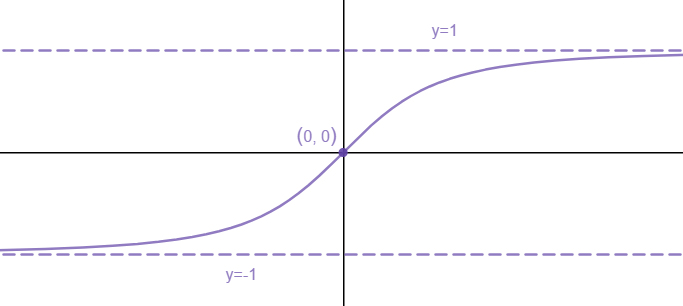
Finally, we can sketch our graph. Let's start with the skeleton. Place all known values down and any asymptotes.

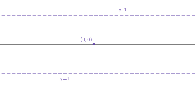
Now given the rest of the information we can sketch.

(Video) Curve Sketching Using Calculus

by PatrickJMT

Here's a video by patrickJMT showing you how to figure out all the necessary information needed to correctly graph a function.

The function he looks at is $$f(x)=\frac{x}{x+4}$$

Domain

When dealing with a rational function the only thing you want to avoid is dividing by zero. Our function becomes undefined when $x=-4$. Therefore, the domain is $(-\infty,-4)$ and $(-4,\infty)$.

Intercepts

To find the $x$ intercepts we set $y=0$. $$\begin{align} \frac{x}{x+4}&=0\\ x&=0 \end{align}$$ So we have an $x$ intercept at $(0,0)$. This is considered a $y$ intercept as well.

Asymptotes

We get vertical asymptotes at any point where the denominator is equal to zero. We already found above that this happens when $x=-4$. So we have a vertical asymptote at $x=-4$.

To find horizontal asymptotes we look at the limit as $x$ approaches infinity and negative infinity. $$\lim_{x\rightarrow\infty}\frac{x}{x+4}=\frac{\infty}{\infty}$$ Because we get infinity over infinity we can apply l'Hospital's Rule. We take the derivative of the numerator and denominator separately and then reapply the limit. $$L'H\Rightarrow\frac{1}{1}=1$$ The limit of a constant is the constant. So we have a horizontal asymptote at $y=1.$

The same result will happen if we test the limit approaching negative infinity.

We can now sketch the skeleton of our graph.

Before we continue notice that, at the vertical asymptote, our function can either go up to infinity or down to negative infinity. To see what our function does we can take the limit at this point from each side. $$\lim_{x\rightarrow-4^-}\frac{x}{x+4}=\infty\\ \lim_{x\rightarrow-4^+}\frac{x}{x+4}=-\infty$$

Increasing and Decreasing

To find the intervals in which our graph is increasing or decreasing we look at the first derivative. \begin{align} f(x)&={x}{x+4}\ f'(x)&=\frac{\color{red}{[x]'}(x+4)-x\color{red}{[x+4]'}}{[x+4]^2}\ &=\frac{(x+4)-x}{(x+4)^2}\ &=\frac{4}{(x+4)^2} \end{align}

Once you have the derivative you need to find where it equals zero or is undefined. You might notice but we get no solution if we set this equal to zero. So let's see where it's undefined, a.k.a. where the denominator equals zero. \begin{align} (x+4)^2&=0\ x+4&=0\ x&=-4 \end{align}

So we can make our sign chart.

Now plug in a value from each interval into the derivative and see what sign the answer is. In this case, if you plug in any number other than $-4$ you get a positive value. So our function is increasing on the intervals $(-\infty,-4)$ and $(-4,\infty)$.

Local Extrema

Since the function is always increasing, there's no local maximum or local minimum.

Concavity

To test concavity we need the second derivative. $$\begin{align} f'(x)&=\frac{4}{(x+4)^2}\\ &=4(x+4)^{-2}\\ f''(x)&=-8(x+4)^{-3}\\ &=\frac{-8}{(x+4)^3} \end{align}$$

Again, we look for where this is equal to zero or undefined. The derivative never equals zero, but it is undefined at $-4$.

So our sign chart is the same as before.

Plug in a value from each interval into the second derivative and note its sign. If we plug in a number below $-4$ we get a negative over a negative which gives a positive. So we know our original function is concave up on this interval. $$(-\infty,-4)\ CU$$

If we plug in a number above $-4$ we get a negative over a positive which gives a negative. So we know our original function is concave down on this interval. $$(-4,\infty)\ CD$$

Sketch

Given all this information we can accurately sketch our graph.

(Video) Using Calculus to Sketch a Curve

by PatrickJMT

Here's another video by patrickJMT in which he sketches a function by figuring out all the different pieces.

The function he looks at is $$f(x)=\sqrt{9-x^2}$$

Domain

Everything under the square root has to be positive. So our domain is any $x$ where $9-x^2\ge0$. The trick to solving quadratic inequalities is to first solve it as an equation. $$\begin{align} 9-x^2&=0\\ x^2&=9\\ x&=\pm3 \end{align}$$ Now make a sign chart with these values.

Now test a value from each interval in the inequality $9-x^2\ge0$. If we plug in a value less than $-3$ we get a negative number which doesn't fit the inequality.

If we plug in a value between $-3$ and $3$ we get a positive value which satisfies our inequality.

Similarly, values above $3$ give us a negative which fails the inequality.

So our domain is $[-3,3]$.

Increase/Decrease

To see where the graph increases and decreases we look at the first derivative. $$\begin{align} f(x)&=\sqrt{9-x^2}\\ f'(x)&=\frac{1}{2\sqrt{9-x^2}}\cdot\color{red}{[9-x^2]'}\\ &=\frac{1}{2\sqrt{9-x^2}}\cdot(-2x)\\ &=\frac{-x}{\sqrt{9-x^2}} \end{align}$$

Now find where the graph equals zero or is undefined. \begin{align} \frac{-x}{\sqrt{9-x^2}}&=0\ -x&=0\ x&=0 \end{align}

The graph is undefined where the denominator is equal to zero. \begin{align} \sqrt{9-x^2}&=0\ 9-x^2&=0\ x^2&=9\ x&=\pm3 \end{align}

So our sign chart contains these three points.

If we plug in a point between $-3$ and $0$ we get a positive over a positive which gives us a positive number. Therefore, the graph is increasing on this interval. $$(-3,0)\ \nearrow$$

If we plug in a point between $0$ and $3$ we get a negative over a positive which gives us a negative number. Therefore, the graph is decreasing on this interval. $$(0,3)\ \searrow$$

Local Extrema

At the point $x=0$ the graph is switching from increasing to decreasing. Therefore, this point will be a local maximum.

Concavity

To find concavity we need to look at the second derivative of the function. $$\begin{align} f'(x)&=\frac{-x}{\sqrt{9-x^2}}\\ f''(x)&=\frac{\color{red}{[-x]'}\sqrt{9-x^2}-(-x)\color{red}{[\sqrt{9-x^2}]'}}{[\sqrt{9-x^2}]^2}\\ &=\frac{-\sqrt{9-x^2}+x\cdot\frac{1}{2\sqrt{9-x^2}}\cdot\color{red}{[9-x^2]'}}{9-x^2}\\ &=\frac{-\sqrt{9-x^2}+\frac{x}{2\sqrt{9-x^2}}\cdot(-2x)}{9-x^2}\\ &=\frac{-\sqrt{9-x^2}-\frac{x^2}{\sqrt{9-x^2}}}{9-x^2}\\ &=-\frac{\sqrt{9-x^2}+\frac{x^2}{\sqrt{9-x^2}}}{9-x^2}\\ &=-\frac{\frac{9-x^2}{\sqrt{9-x^2}}+\frac{x^2}{\sqrt{9-x^2}}}{9-x^2}\\ &=-\frac{\frac{9}{\sqrt{9-x^2}}}{9-x^2}\\ &=-\frac{9}{(9-x^2)^{\frac32}}\\ \end{align}$$

Next, find where the second derivative equals zero or is undefined. If you can't tell already, we will get no solution if we set this equal to zero. So that just leaves finding where its undefined. We look at where the denominator equals zero. \begin{align} (9-x^2)^{\frac32}&=0\ 9-x^2&=0\ x^2&=9\ x&=\pm3 \end{align}

So our sign chart looks like this.

There's only one interval and when we test a number inside it, we get a negative answer. This means our original function is concave down over this entire interval.

Sketch

With all this information we can accurately sketch our graph.