Статистика радіоактивного розпаду

Activity - the rate of radioactive decay

The activity of a radioactive substance denotes how quickly it will shed mass (to reach a more stable binding energy per nucleon) or energy. Since activity is a function of time, this rate of decay decreases as the substance's total population also decreases.

In other words, as more of the substance decays with time, the slower it decays.

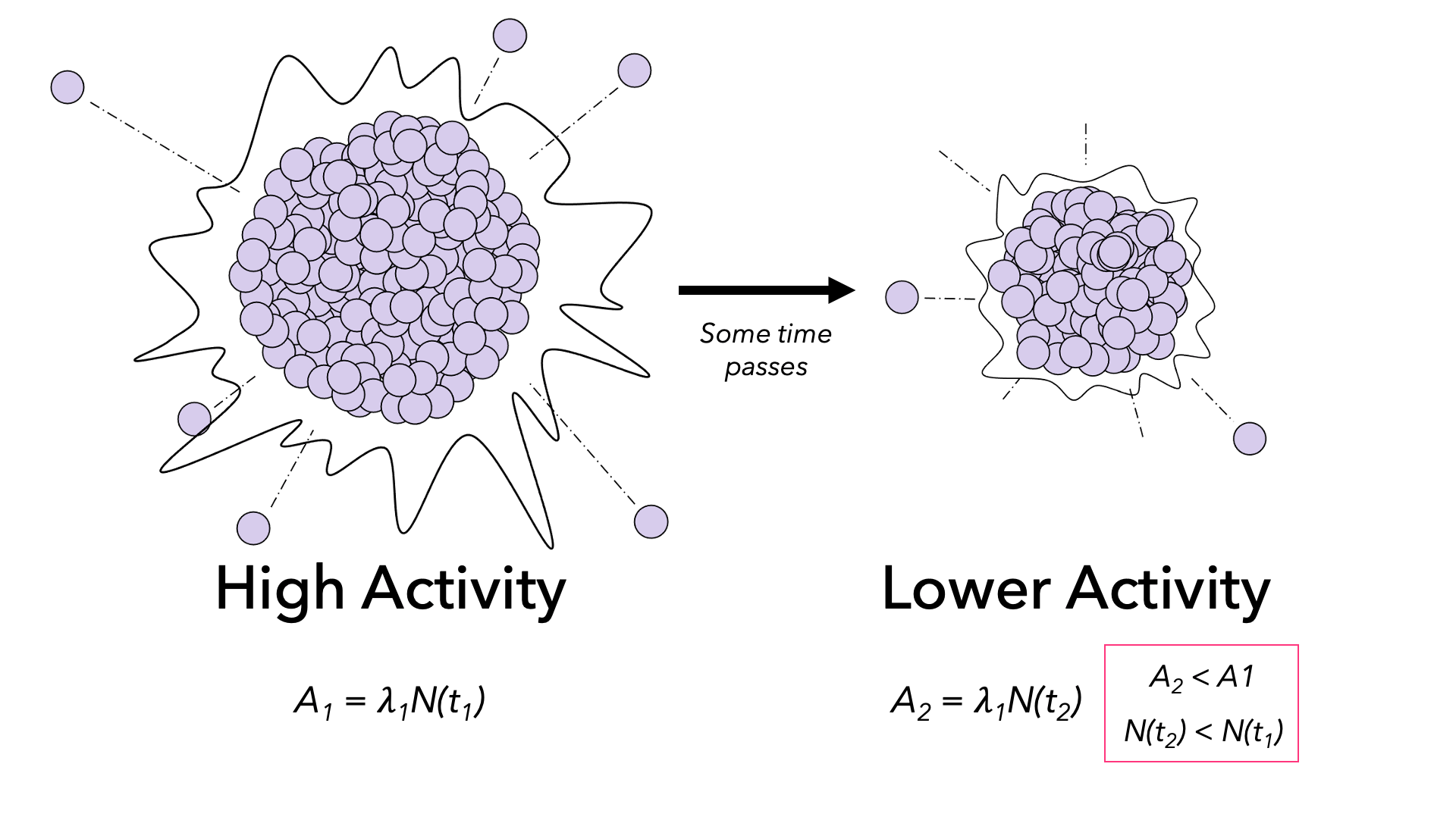
Imagine you're looking at a radioactive element. Let's say we zoom in. Now, we're looking at one atom. Will it decay? You know that it will eventually. But you don't know if it will take one second or 100 million years. There is no way to tell when an individual atom will decay. So, how do we study the decay rates? We use statistics! We examine the decay of large samples and look at the averages. It's similar to chemical kinetics!

A Quick Refresher on Kinetics

It's helpful to have a quick refresher on kinetics. Do you remember what kinetics is? It's the study of reaction rates. To describe rates, we wrote rate laws. They mathematically linked the reactants' concentrations and the reaction rate. The exponents in the equation told us the reaction order. For a zero-order reactant, changing its concentration didn't affect the rate. A first-order reactant had a one-to-one effect. So, doubling the concentration doubled the rate. A second-order reactant was exponential. Doubling the reactant's concentration quadrupled the rate. It turns out that all radioactive decay is first order.

Differences for Radioactivity

We also studied factors affecting reaction rates. For example, increasing the temperature increases the reaction rate. Why? Because we are increasing the average kinetic energy. So, we have more collisions. The same reasoning applied to pressure, surface area, and concentration. We also saw the same effects from catalysts because they lower activation energy. None of these apply to radioactive decay. Why? In some ways, atoms and molecules behave similarly to our macroscopic world. But, nuclei and subatomic particles are too small. At the subatomic level, everything is moving or vibrating near the speed of light. We don't have conventional ways to alter them. They are entirely unaffected by their surroundings.

Decay Equation for Radioactivity

Let's take a look at the rate equation that governs radioactive decay.

$A=\lambda\times N$

You'll notice that this doesn't look like our rate equations from kinetics. First, what in the world is A? It's the activity and has units of decays per time. The most common units are the Baquerell ($1\,\frac{decays}{s}$) and the Curie ($3.7\times10^{10} \frac{decays}{s}$). You'll also notice that there are no concentrations. Why? We aren't working with solutions. It's far easier to work in the number of atoms. That's the N in the equation. In practice problems, you might have the mass of a sample. You'll need to use the molar mass to convert it to moles. Then use Avagadro's number to convert moles to atoms. Finally, what's $\lambda$. That's the decay constant, lambda! It's units are per second ($\frac{1}{s}$). Thankfully, nuclear chemists have calculated it for most radioactive isotopes. So, you can look it up and use it!

Using the Decay Equation

Let's look at a few examples of using the decay equation.

1. 0.0169 grams of potassium-40 undergoes $4400 \frac{decays}{sec}$. What is potassium-40's decay constant?

First, we need to convert grams to moles and then atoms. We can use dimensional analysis.

$0.0169g \times \frac{1 mol}{39.93 g} \times 6.022\times10^{23}\frac{atoms}{mol} =2.55\times10^{20} atoms$

Now, we can plug $N$ and $A$ into our formula. We are solving for $\lambda$.

$4400 \frac{decays}{sec}=2.55\times10^{20} atoms \times \lambda \rightarrow \lambda= \frac{4400}{2.55\times 10^{20}}= \frac{1.73\times10^{-17}}{s}$

The units seem a little strange. But, in the Bequerell, the decays are atoms decaying. So, atoms and decays will cancel. The constant is in per second.

1. Using potassium-40's decay constant, calculate the activity of 1.00 grams.

Like the last problem, we need to convert grams to moles and then moles to atoms.

$1.00g \times \frac{1 mol}{39.93 g} \times \frac{6.022\times10^{23}atoms}{mol}=1.51\times 10^{22} atoms$

Next, we can plug $\lambda$ and the number of atoms into the decay equation.

$A=\lambda \times N = \frac{1.73\times10^{-17}}{s} \times 1.51\times 10^{22} atoms = 260755.51\frac{decays}{s}$

Another Kinetic Refresher: First-Order Differential Rate Law

All radioactive decay is first order. That means we can apply the first-order differential and integrated rate laws. Remember, the differential rate law lets us compare concentrations at a specific time. The general form is $ln{(\frac{[A]}{[A]_{o}})}=-k\times t$. Let's apply this to a radioactivity problem!

1. The decay constant for Carbon-14 is $\frac{3.84\times10^{-12}}{sec}$. If we have a 5.50-gram sample, how much remains after one-thousand years?

Since we have the decay constant, we can use the differentiated rate law to calculate our change.

$\ln{(\frac{A}{A_{o}})}=-\lambda(t) \rightarrow\ln{(\frac{A}{5.50g})}=-\frac{3.84\times10^{-12}}{sec}\times 3.154\times10^{10} sec \rightarrow \ln{(\frac{A}{5.50g})}=-0.12$

$A=5.50\times e^{-0.12}= 4.87g$

Half-lives of Radioactive Elements

We can also use the differentiated rate law to calculate the half-life. As an example, let's use carbon-14 again.

Remember, the half-live occurs when $\ln{(\frac{A}{A_{o}})}=\ln{(0.5)}=-0.693$.

$-0.693=-\lambda\times t \rightarrow t=\frac{-0.693}{\frac{-3.84\times10^{-12}}{sec}}\rightarrow t=180507078271 sec \rightarrow t=5724 yrs$

We focussed on the half-life of carbon-14 because in a future lesson we'll explore radioactive dating.

Does the Type of Decay Matter?

Previously we studied the different types of radioactive decay. We examined alpha, beta, gamma, and electron capture. We might expect that different types of decay methods would affect the half-life. But, it doesn't. For example, when we studied decay series we examined the actinide isotope Thorium-232. It has a half-life of 14 gigayears. But, one of its granddaughters, Radon-220 has a half-life of 55 seconds. Both undergo alpha decay. So, we see that the half-life depends on nuclear stability and binding energy.

(Video) 20.4 Kinetics of Nuclear Decay | General Chemistry

by Chad's Prep

In this video, Chad explains the kinetic of nuclear decay. He starts with a quick refresher on first-order decay and half-life. Then, you'll get to see examples of the most common half-life problems. Finally, he applies the half-life equations to radioactive dating. Are you struggling with radioactive decay rates? This video will help!